Examining the centrality of trait absorption
knitr::include_graphics("/img/traits.jpg", error = FALSE)
Summary
In this blog, I analyse the human trait of becoming absorbed in relation to several other traits. Complementary to factor analysis, which is the most commonly applied method used to explain the interrelationships between multiple traits, here network analysis is used to provide alternative, additional insights into the function and meaning of absorption amidst other traits. The findings contribute to the debate whether or not traits are best understood in terms of underlying latent variables or perhaps in terms of a network.
Absorption describes the susceptibility to enter psychological states that restructure or alter our everyday experience. These more or less transient states may have a dissociated character or an integrative and peak-experience-like quality. Correspondingly, they may have a “sentient” external focus, or else may reflect an inner focus on reminiscences, images, and imaginings” (Tellegen, 1992). For long, the Tellegen Absorption Scale (TAS) is the most-widely used self-report questionnaire that measures this trait (Tellegen & Atkinson, 1974; Tellegen, 1981), used in a large variety of contexts, including hypnosis and music.
To examine the role and mechanisms of trait absorption, Tellegen (1992) advocated a multivariate approach by using the absorption scale together with other personality measures. Indeed, although absorption naturally varies from person to person, it often varies unmistakably as a function of other personality characteristics.
The question what the psychological construct of personality is informs on the kind of statistical model that is applicable. Traditionally, latent variables as underlying common causes for personality have been used (left figure). On the other hand, Mottus and Allerhand (2017) recently discussed in “Why Do Traits Come Together? The Underlying Trait and Network Approaches” how one’s overall identity can also be conceived as a dynamical system of interconnected personality characteristics (right figure). According to these authors, “compared with the underlying trait approach, the network approach allows for a richer way of representing associations between personality characteristics and their associations with variables outside the personality domain” (p.140).
# Example of an reflective model
M.1A <- matrix(0, 11, 11)
M.1A[1, 2] <- M.1A[1, 3] <- M.1A[1, 4] <- M.1A[1, 5] <- M.1A[1, 6] <- M.1A[1, 7] <- M.1A[1, 8] <- M.1A[1, 9] <- M.1A[1, 10] <- M.1A[1, 11] <- .25
gr.1 <- list(1, 2:11)
names1 <- c("ID", 1:10)
# Example of an network model
M.1C <- matrix(0, 10, 10)
M.1C[1, 3] <- M.1C[2, 1] <- M.1C[2, 4] <- M.1C[2, 5] <- M.1C[2, 3] <- M.1C[2, 6] <-
M.1C[2, 6] <- M.1C[5, 2] <- M.1C[3, 2] <- M.1C[3, 6] <- M.1C[1, 1] <- M.1C[5, 5] <-
M.1C[8, 8] <- M.1C[7, 7] <- M.1C[9, 9] <- M.1C[6, 10] <- M.1C[6, 8] <-
M.1C[6, 7] <- M.1C[10, 9] <- .25
layout(t(1:2))
A <- qgraph::qgraph(M.1A, border.width = c(3, rep(3, 10)), border.color = "#FFD700", asize = 6, vsize = c(8, rep(12, 10)), label.color = "black", color = "#FFD700", maximum = .5, labels = names1, theme = "colorblind")
C <- qgraph::qgraph(M.1C, border.width = 3, border.color = "#FFD700", asize = 6, vsize = 8, label.color = "black", color = "#FFD700", maximum = .5, layout = "spring", theme = "colorblind")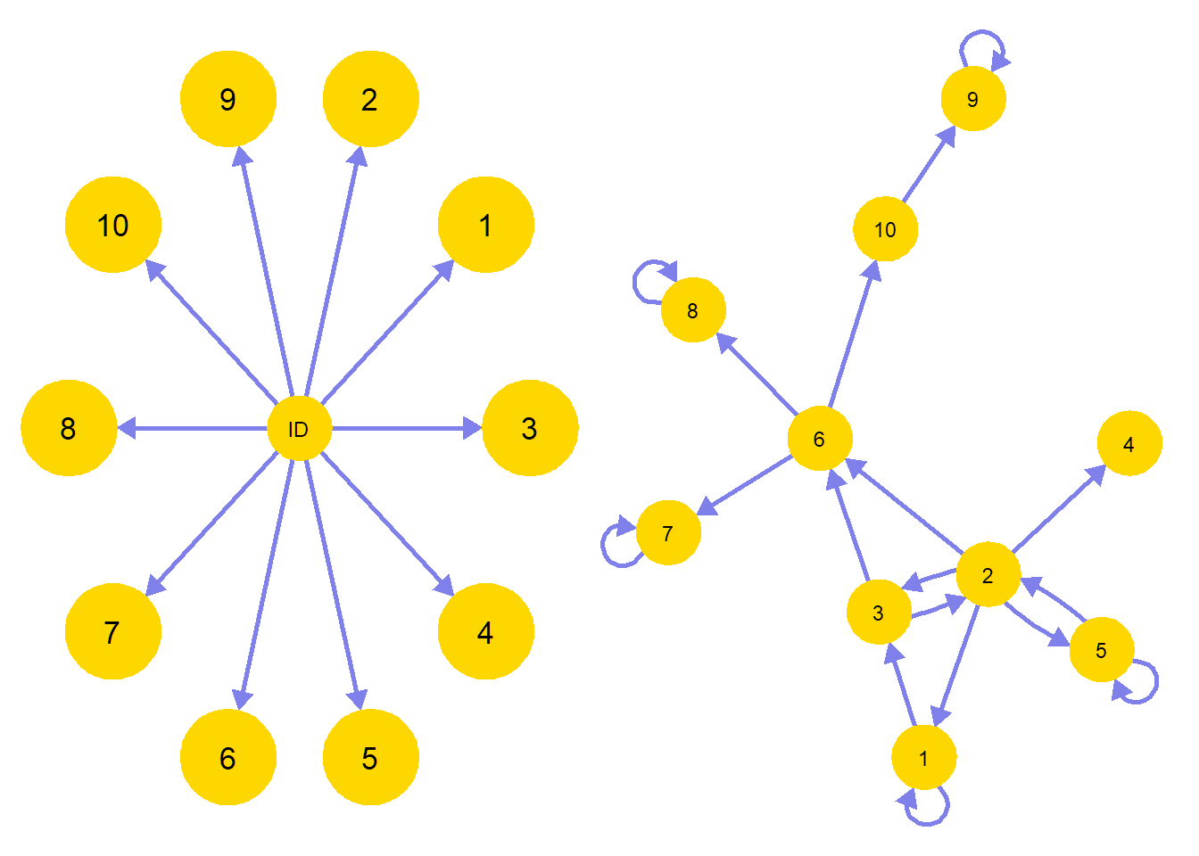 Let’s follow this approach and adopt a network perspective to the analysis of the TAS amidst other personality traits, and compare it with the more traditional factor modeling approaches used to analyse the relations between multiple traits.
Question
How does trait absorption function within a larger network of personality traits, and what are the dynamics of traits mutually affecting each other?
Answering this question helps us to understand which traits are conditionally related to each other, and we can use network analysis to help us answer it!
Note that, even if you’re not specifically interested in absorption, this is still a useful analysis because it will tell you how to apply psychometric network analysis based on summary data and shows how to compare network models with factor models. Let’s get started!
Libraries
Load the following libraries. If you have never used one of htese packages, you will need to install with, for example, install.packages("relaimpo").
library(tidyverse)
library(relaimpo)
library(matrixcalc)
library(EFAtools)
library(psychonetrics)
library(semPlot)
library(qgraph)
# library(dplyr)
library(corrplot)
library(lattice)
library(networktools)
library(bnlearn)
library(Rgraphviz)
library(pcalg)
library(BayesNetBP)
# require(RBGL)
require(reshape2)

set.seed(123)
Data
We use data from an article by Kumar, Pekala and Cummings (1996) entitled Trait factors, state effects, and hypnotizability. As part of this study, factor analysis was conducted to examine how 15 personality traits, including absorption as measured by the Tellegen Absorption Scale (TAS; See Tellegen & Atkinson, 1974), clustered together on underlying, latent factors. The results suggested three, general trait factors: absorption-permissiveness, general sensation seeking, and social desirability.
Although the raw data are not available any more, we can nonetheless retrieve and calculate the implied correlation matrix from the factor loadings and factor-intercorrelations reported in the paper. To do so, we need to use some matrix algebra. The following code is shown so you can see how this works.
Let the matrix of factor loadings be “L” and “F” the inter-factor correlation matrix. The implied correlation matrix (Σ) is then given using the following equation, with “L’” representing the transposed matrix of L:
Σ = LFL′
Let’s read in the factor loadings printed as a table from the 1996 paper.
L <- matrix(c(
  0.075, 0.357, 0.33,
  0.294, 0.316, 0.298,
  -0.017, 0.488, -0.079,
  -0.101, 0.79, -0.045,
  0.763, 0.028, 0.17,
  0.773, -0.114, 0.197,
  0.76, 0.073, 0.045,
  0.806, -0.05, -0.307,
  0.719, 0.005, -0.018,
  0.417, 0.214, -0.089,
  0.687, -0.152, 0.14,
  -0.044, -0.002, 0.575,
  0.23, -0.065, 0.404,
  0.684, -0.009, -0.067,
  -0.1, -0.274, 0.382
), nrow = 15, ncol = 3, byrow = TRUE)

colnames(L) <- paste0("F", 1:3)
rownames(L) <- paste0("V", 1:15)

# Labels
varLabs <- c(
  "Thrill and adventure seeking",
  "Experience seeking",
  "Boredom susceptibility",
  "Disinhibition",
  "TAS",
  "Peak experiences",
  "Dissociated experiences",
  "Openness to inner experiences",
  "Belief in supernatural",
  "Emotional extraversion",
  "Intrinsic arousal",
  "Ego strength",
  "Intellectual control",
  "Cognitive regression",
  "Social desirability"
)
The second data frame contains information about the factor intercorrelations as reported in the text of the paper.
F <- matrix(c(
  1, 0.225, 0.203,
  0.225, 1, -0.079,
  0.203, -0.079, 1
), nrow = 3, ncol = 3, byrow = TRUE)

colnames(F) <- rownames(F) <- paste0("F", 1:3)
Next, we apply the formula just presented. To clarify: We enforce the diagonal to be 1 with diag(R) <- 1. This diagonal of the implied correlation matrix holds the commmunalities (i.e., the explained variances). These will only be 1 if the factor loading structure exactly reproduces the observed correlations (which is rarely the case in empirical data). Thus, to get a proper correlation matrix, the diagonal is replaced with 1’s.
# \[ $S = {LFL'} \]
# $$S = LFL'$$
R <- L %*% F %*% t(L)
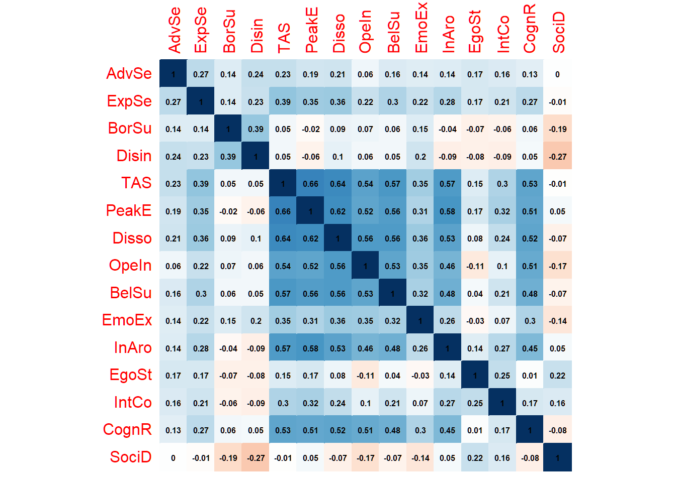
diag(R) <- 1This gives us the following correlation matrix:
# Short Labels
colnames(R) <- rownames(R) <- c("AdvSe", "ExpSe", "BorSu", "Disin", "TAS", "PeakE", "Disso", "OpeIn", "BelSu", "EmoEx", "InAro", "EgoSt", "IntCo", "CognR", "SociD")

corrplot(R,
  method = "color", addCoef.col = "black",
  number.cex = .5, cl.pos = "n", diag = T, insig = "blank"
)
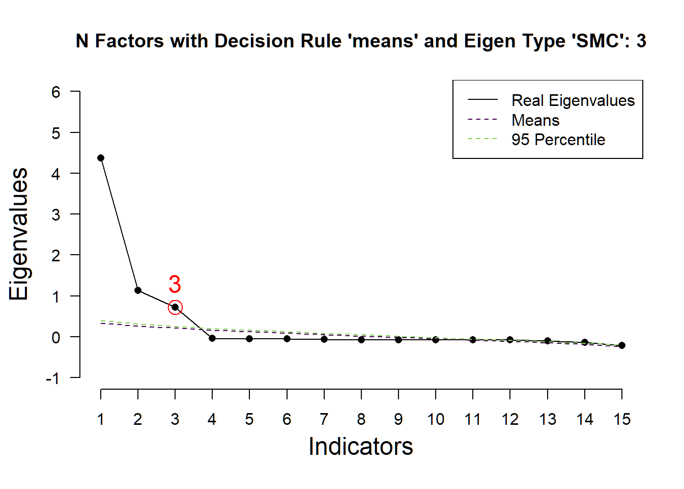
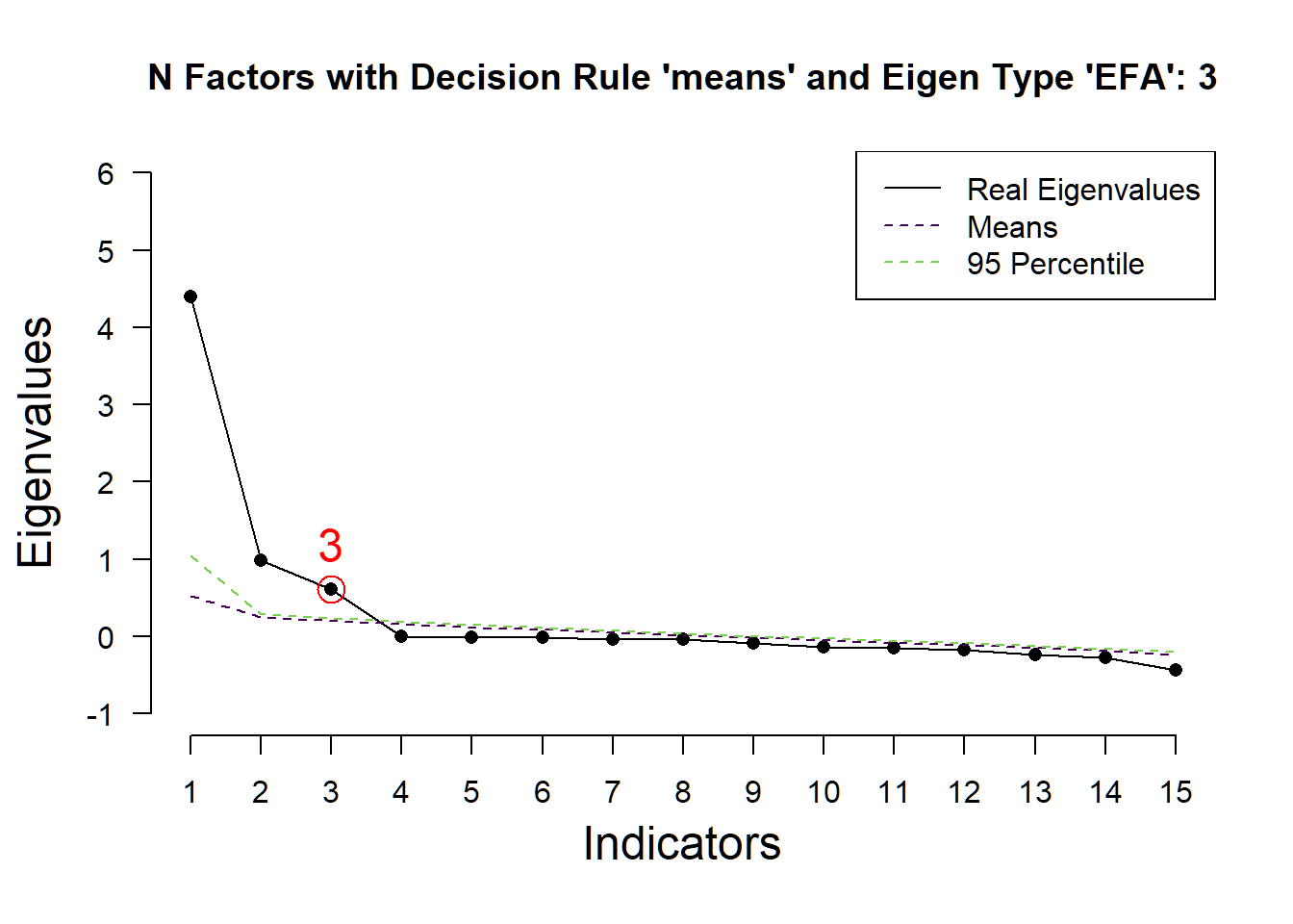
Next, we’ll perform exploratory factor analysis to double-check our derived correlation matrix. We examinethe amount of factors, factor loadings and factor intercorrelations, using the information in the paper by Pekala et al. on choosing the appropriate extraction method (“maximum likelihood”), sample size (“n=523”), and rotation technique (“quartimin”).
# number of factors
nfac_all <- N_FACTORS(R, N = 523, method = "ML")
##
(*) <U+0001F3C3> ( ) ( ) ( ) ( ) ( ) Running EKC
(*) (*) <U+0001F3C3> ( ) ( ) ( ) ( ) Running HULL
(*) (*) (*) <U+0001F3C3> ( ) ( ) ( ) Running KGC
(*) (*) (*) (*) <U+0001F3C3> ( ) ( ) Running PARALLEL
(*) (*) (*) (*) (*) <U+0001F3C3> ( ) Running SCREE
(*) (*) (*) (*) (*) (*) <U+0001F3C3> Running SMT
(*) (*) (*) (*) (*) (*) (*) Done!nfac_all##
## -- Tests for the suitability of the data for factor analysis -------------------
##
## Bartlett's test of sphericity
##
## v The Bartlett's test of sphericity was significant at an alpha level of .05.
## These data are probably suitable for factor analysis.
##
## <U+0001D712>²(105) = 2480.17, p < .001
##
## Kaiser-Meyer-Olkin criterion (KMO)
##
## v The overall KMO value for your data is marvellous with 0.91.
## These data are probably suitable for factor analysis.
##
## -- Number of factors suggested by the different factor retention criteria ------
##
## ( ) Comparison data: NA
## ( ) Empirical Kaiser criterion: 3
## ( ) Hull method with CAF: 1
## ( ) Hull method with CFI: 3
## ( ) Hull method with RMSEA: 3
## ( ) Kaiser-Guttman criterion with PCA: 3
## ( ) Kaiser-Guttman criterion with SMC: 2
## ( ) Kaiser-Guttman criterion with EFA: 1
## ( ) Parallel analysis with PCA: 3
## ( ) Parallel analysis with SMC: 3
## ( ) Parallel analysis with EFA: 3
## ( ) Sequential <U+0001D712>² model tests: 3
## ( ) Lower bound of RMSEA 90% confidence interval: 2
## ( ) Akaike Information Criterion: 3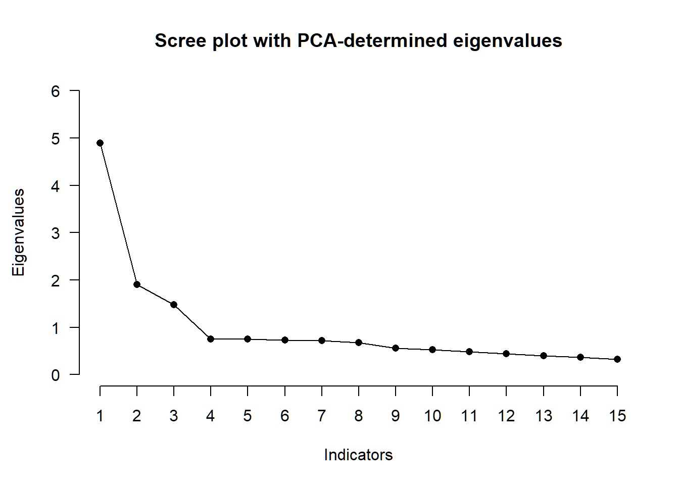

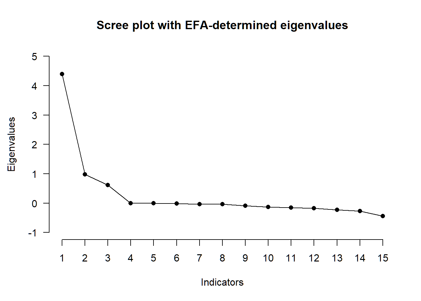
x <- PARALLEL(R, N = 523, method = "ML")
plot(x)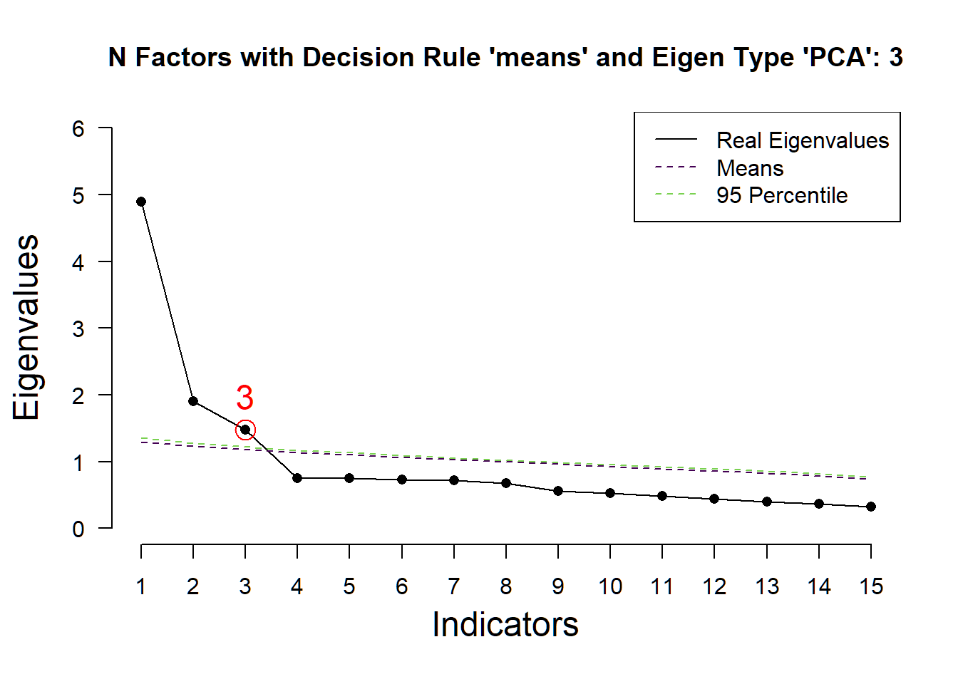
spss_ml <- EFA(R, n_factors = 3, N = 523, type = "SPSS", method = "ML", rotation = "quartimin")
spss_ml
##
## EFA performed with type = 'SPSS', method = 'ML', and rotation = 'quartimin'.
##
## -- Rotated Loadings ------------------------------------------------------------
##
## F1 F2 F3
## AdvSe .074 .357 .330
## ExpSe .293 .317 .298
## BorSu -.018 .488 -.079
## Disin -.103 .790 -.045
## TAS .762 .031 .170
## PeakE .773 -.111 .197
## Disso .759 .076 .045
## OpeIn .805 -.046 -.307
## BelSu .718 .008 -.018
## EmoEx .416 .216 -.089
## InAro .687 -.149 .140
## EgoSt -.044 -.003 .575
## IntCo .230 -.065 .404
## CognR .683 -.006 -.067
## SociD -.099 -.275 .382
##
## -- Factor Intercorrelations ----------------------------------------------------
##
## F1 F2 F3
## F1 1.000 0.223 0.203
## F2 0.223 1.000 -0.078
## F3 0.203 -0.078 1.000
##
## -- Variances Accounted for -----------------------------------------------------
##
## F1 F2 F3
## SS loadings 4.436 1.294 0.858
## Prop Tot Var 0.296 0.086 0.057
## Cum Prop Tot Var 0.296 0.382 0.439
## Prop Comm Var 0.673 0.196 0.130
## Cum Prop Comm Var 0.673 0.870 1.000
##
## -- Model Fit -------------------------------------------------------------------
##
## <U+0001D712>²(63) = 0.00, p = 1.000
## CFI = 1.00
## RMSEA [90% CI] = .00 [.00; .00]
## AIC = -126.00
## BIC = -394.35
## CAF = .50Convert to matrix format
calc_matrix <- round(
  matrix(spss_ml$rot_loadings,
    nrow = 15,
    ncol = 3
  ),
  2
)

## Plot correlation matrices
par(mfrow = c(1, 3))
corrplot(calc_matrix,
  method = "color", addCoef.col = "black",
  number.cex = .9, cl.pos = "n", diag = T, insig = "blank"
)
title(main = "Estimated matrix")
corrplot(abs(L - calc_matrix),
  method = "color", addCoef.col = "black",
  number.cex = .9, cl.pos = "n", diag = T, insig = "blank"
)
title(main = "Absolute Difference")
corrplot(L,
  method = "color", addCoef.col = "black",
  number.cex = .9, cl.pos = "n", diag = T, insig = "blank"
)
title(main = "Original factor loadings")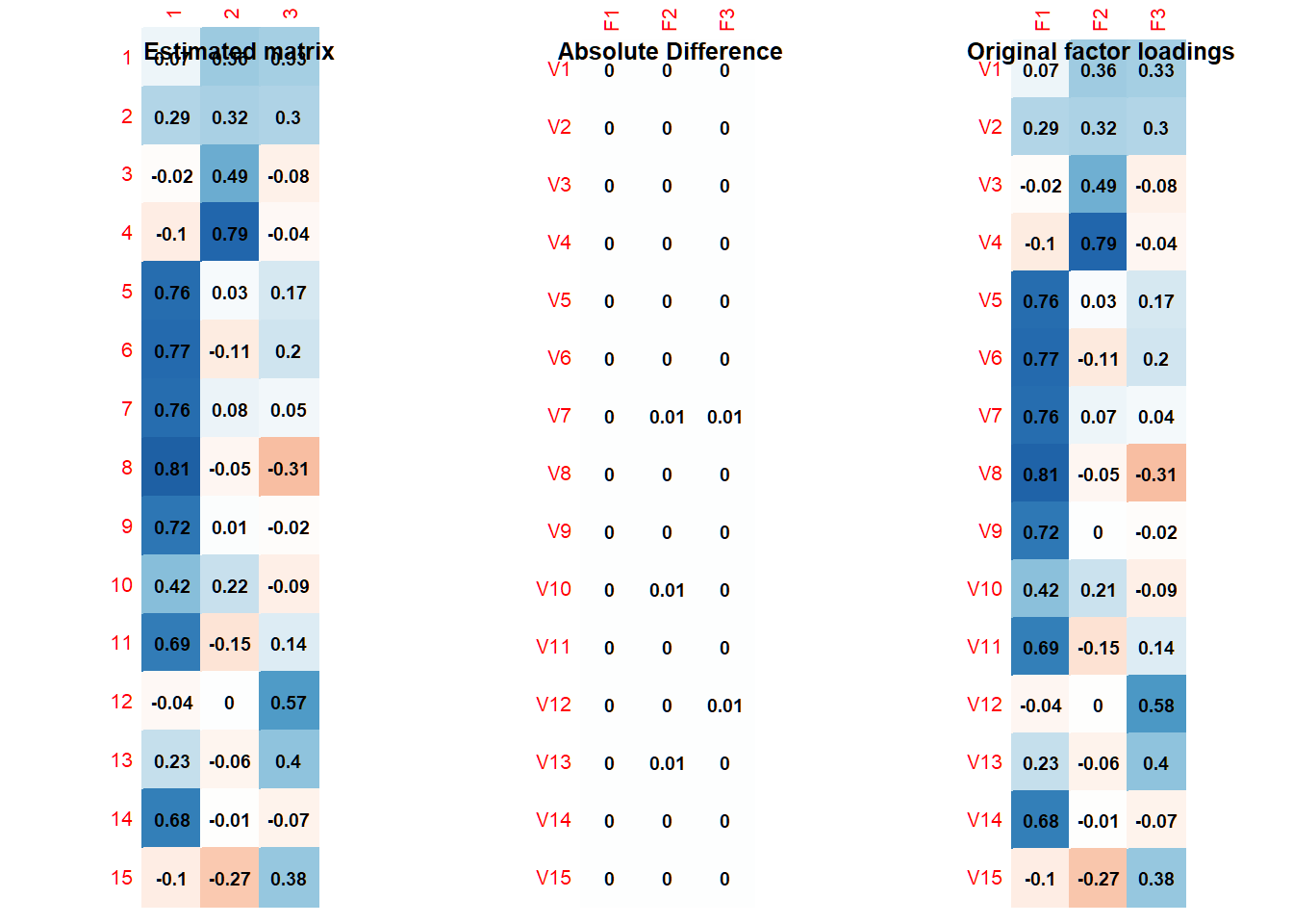
As the results show, we reproduce almost exactly the same factor loadings and interfactor correlation matrix as the ones with which we began. This indicates that we retrieved the correct correlation matrix. The matrix is positive definite:
is.positive.definite(round(R, 2))## [1] TRUELast, we need to identify whether there are any redundant variables, that is: whether two or more measures are actually the same construct. One tool for this is the goldbricker function as part from the networktools package. For every pair of variables, this tool examines whether their correlations with all other variables are similar to each other.
This function requires full data, though. Hence, on the basis of the correlation matrix, we first need to simulate raw data so that we can use the goldbricker function.
Simulating data
One way to simulate data from the correlation matrix only is through Cholesky decomposition. Since our goal is to obtain simulated raw data that reproduces the correlation matrix as closely as possible, we need to identify the seed with which the difference is minimized.
minvalue <- 50
minseed <- 9000

for (i in 35000:40000) {
  set.seed(i)
  M <- chol(R)
  r <- t(M) %*% matrix(rnorm(15 * 523), nrow = 15, ncol = 523)
  r <- t(r)

  rdata <- as.data.frame(r)
  corrdata <- round(cor(rdata), 3)

  diff <- abs(R - corrdata)
  diff2 <- diff > 0.05

  sumdiff <- sum(diff2)

  # updating minimal value
  minvalue <- ifelse((sumdiff < minvalue), sumdiff, minvalue)
  minseed <- ifelse((sumdiff <= minvalue), i, minseed)
}
The values are:
minvalue## [1] 6minseed## [1] 38022The results above suggested that with setting the seed at 38022, we simulate data with which we reproduce the correlation matrix as closely as possible with only 6 coefficients that differ more than 0.05.
set.seed(minseed)

M <- chol(R)
nvars <- dim(M)[1]

# number of observations to simulate
nobs <- 523

# Random variables that follow the R correlation matrix
r <- t(M) %*% matrix(rnorm(nvars * nobs), nrow = nvars, ncol = nobs)
r <- t(r)
rdata <- as.data.frame(r)
rrdata <- round(cor(rdata), 3)

diff <- abs(R - rrdata)
diff2 <- diff > 0.05
sum(diff2)
## [1] 6Let’s plot the absolute differences:
corrplot(abs(R - rrdata),
method = "color", addCoef.col = "black",
number.cex = .6, cl.pos = "n", diag = T, insig = "blank"
)
title(main = "Absolute Difference")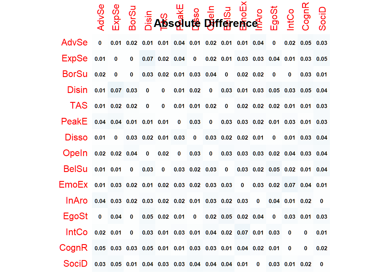 With the simulated data at hand, we can now check for variable/ node redundancy.
badpairs <- goldbricker(rdata, p = 0.05, method = "hittner2003", threshold = 0.20, corMin = 0.5, progressbar = FALSE)badpairs## Suggested reductions: Less than 20 % of correlations are significantly different for the following pairs:
## PeakE & TAS Disso & TAS
## 0.1538462 0.1538462These findings suggest that the self-reports questionnaires used to assess peak experiences, absorption and dissociation actually have measured the same underlying construct. Since we are specifically interested in trait absorption here, we therefore choose, for now, to remove peak experiences and dissociation.
R13 <- R %>%
  as.data.frame() %>%
  dplyr::select(-PeakE, -Disso) %>%
  slice(-6, -7) %>%
  as.matrix()
Network Analysis
Next, we make use of three different, yet complementary types of network analyses: Gaussian graphical model, Relative importance network, and Bayesian networks
Gaussian graphical model
First, a sparse Gaussian graphical model (GGM) is computed using graphical lasso based on extended BIC criterium. The tuning parameter is chosen using the Extended Bayesian Information criterium (EBIC).
graph <- EBICglasso(R13, n = 523, gamma = 0.5)
g <- qgraph(graph, layout = "spring", title = "GGM with EBICglasso", details = TRUE)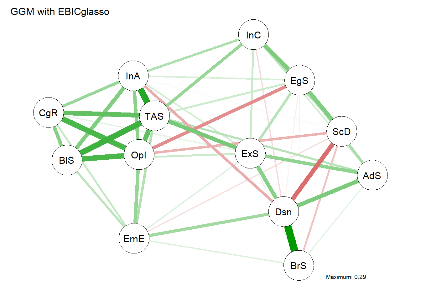 And the corresponding centrality plot. Note that the centrality plot uses z-scores on the x-axis, which indicates each node’s centrality compared to the mean centrality.
# plot centrality plot
centralityPlot(EBIC = graph, scale = "z-scores", include = c("ExpectedInfluence"))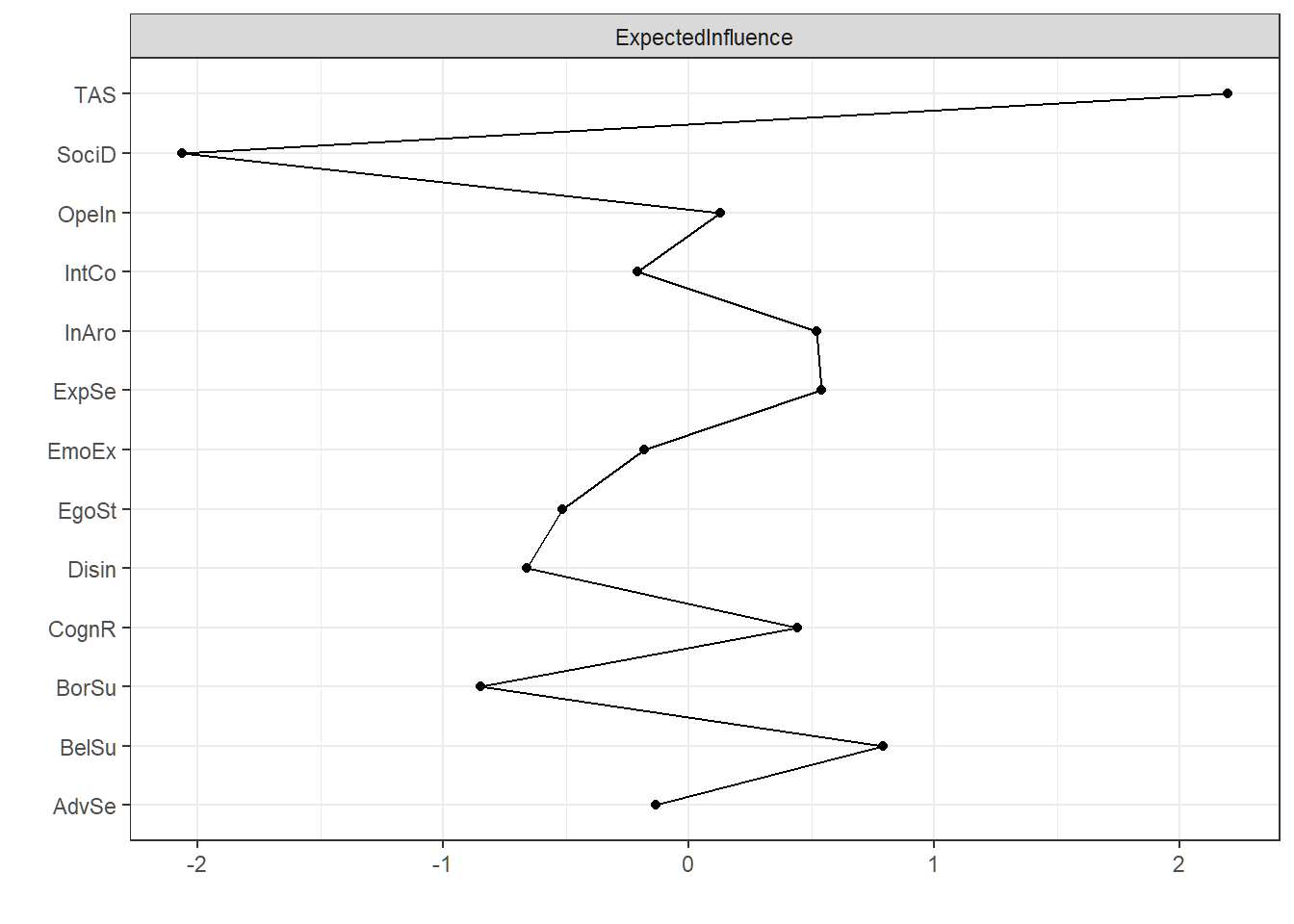 As the plot shows, absorption as measured with the TAS is clearly the most central node in the network of traits.
Relative importance network
Next, we estimate a relative importance network to further examine which trait is the most central. Here, we use the relaimpo package.
rownames(R13) <- colnames(R13)
names.sub <- colnames(R13)

# relmat will contain the weights matrix of the relative importance network
relmat <- matrix(0, 13, 13)

# r2vec will contain the predictability scores
r2vec <- numeric(13)

# function needed to reorder the matrix according to "names"
reorder_mat <- function(matrix, names) {
  if (is.null(dimnames(matrix))) {
    stop("Error: matrix must have dimension names")
  }
  if (!all(rownames(matrix) %in% names)) {
    stop("Error: dimnames(matrix) does not match names")
  }
  matrix[names, names]
}
When using the relaimpo package with a correlation matrix, we need to reorder the correlation matrix so that we loop through all variables once, to ensure that each of the variables appears as the first column in the matrix once (functioning as the y-variable) and all other variables as predictors (x-variables). We then calculate the relative importance and predictability.
for (i in 1:13)
{
  # reorder variables so each, in turn, is first in the matrix
  temp <- reorder_mat(R13, c(names.sub[i], names.sub[seq(1:13)[-i]]))

  # then estimate relative importance for each variable
  relmat[seq(1:13)[-i], i] <- calc.relimp(temp, type = "lmg", rela = TRUE)$lmg

  # and the predictability of each variable
  r2vec[i] <- calc.relimp(temp)$R2
}
relimpnet_c <- as.table(apply(relmat, 2, as.numeric))

# for clarity purposes, we delete all edges below 0.05
relimpnet_censored <- ifelse(relimpnet_c < 0.05, 0, relimpnet_c)
Let’s plot the network
relimpnet_plot <- qgraph(relimpnet_censored, labels = names.sub, title = "censored graph", repulsion = .8, asize = 5, pie = r2vec)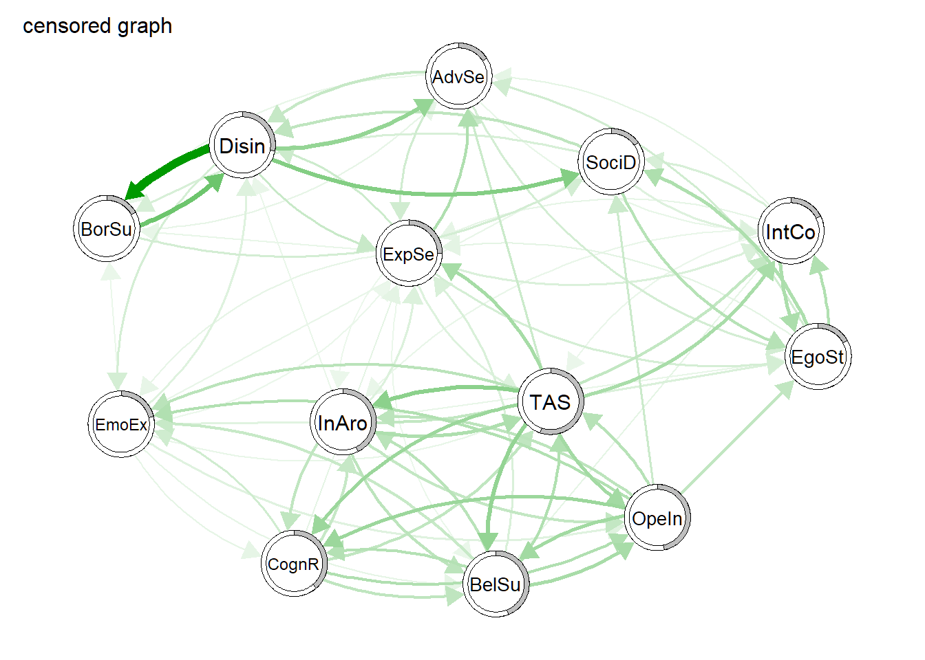
We also plot the corresponding centrality values. Since the relative importance network is a directed network, we now have outstrength and instrength as measures of centrality.
centralityPlot(relimpnet_plot)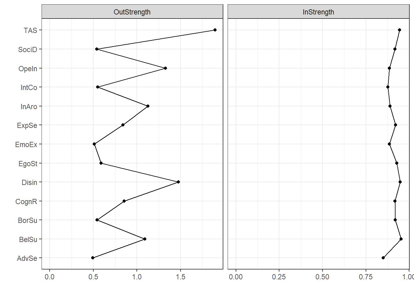
Bayesian network
last, we estimate a Bayesian network in the form of a Directed Acyclical Graph (DAG). To do so, we use the bnlearn package. Because the algorithms in bnlearn only accept n*p dataframes, we’ll make use of our previously simulated data again. First, we remove the nodes that we identified earlier as being redundant to absorption.
rdata2 <- rdata %>% dplyr::select(-PeakE, -Disso)Next, we learn the structure of the Bayesian network using a hill-climbing (hc) search. The hc algorithm is found to be one of the better performing algorithms as compared to other structure learning algorithms.
For model averaging purposes, we use R = 100 (the amount of bootstrapped networks) and for computation purposes keep the pertubations relatively low.
set.seed(38022)

bootnet <- boot.strength(rdata2,
  R = 100,
  algorithm = "hc",
  debug = FALSE,
  algorithm.args = list(restart = 5, perturb = 10)
)
We then use the optimal cutpoint to obtain the averaged network structure (Scutari & Nagarajan, 2013).
avgnet <- averaged.network(bootnet)
avgnet
##
## Random/Generated Bayesian network
##
## model:
## [Disin][TAS][EgoSt][AdvSe|Disin:TAS:EgoSt][BorSu|Disin][BelSu|TAS]
## [SociD|Disin:EgoSt][ExpSe|AdvSe:TAS][OpeIn|TAS:BelSu:EgoSt:SociD]
## [InAro|ExpSe:Disin:TAS:OpeIn:BelSu][IntCo|TAS:InAro:EgoSt:SociD]
## [CognR|TAS:OpeIn:BelSu:InAro][EmoEx|Disin:TAS:OpeIn:CognR]
## nodes: 13
## arcs: 30
## undirected arcs: 0
## directed arcs: 30
## average markov blanket size: 6.77
## average neighbourhood size: 4.62
## average branching factor: 2.31
##
## generation algorithm: Model Averaging
## significance threshold: 0.5avgnet$learning## $whitelist
## NULL
##
## $blacklist
## NULL
##
## $test
## [1] "none"
##
## $ntests
## [1] 0
##
## $algo
## [1] "averaged"
##
## $args
## $args$threshold
## [1] 0.5# Compute the score of the Bayesian network
score(avgnet, data = rdata2) # -9025## [1] -9025.184thresh <- avgnet$learning$args[[1]]
thresh # optimal significance threshold = 0.5## [1] 0.5astr <- arc.strength(avgnet, rdata2, "bic-g") ## compute edge strengths
astr## from to strength
## 1 AdvSe ExpSe -8.3613655
## 2 ExpSe InAro -1.9279204
## 3 Disin AdvSe -15.7069354
## 4 Disin BorSu -46.5266458
## 5 Disin EmoEx -6.3703300
## 6 Disin InAro -9.7175866
## 7 Disin SociD -8.0229325
## 8 TAS AdvSe -8.2927780
## 9 TAS ExpSe -35.9732318
## 10 TAS OpeIn -27.8920299
## 11 TAS BelSu -99.0628213
## 12 TAS EmoEx -2.9700347
## 13 TAS InAro -20.4333814
## 14 TAS IntCo -6.0132996
## 15 TAS CognR -13.7617597
## 16 OpeIn EmoEx -6.8310946
## 17 OpeIn InAro -12.7745380
## 18 OpeIn CognR -4.2732885
## 19 BelSu OpeIn -37.5382008
## 20 BelSu InAro -0.8181870
## 21 BelSu CognR -1.7031832
## 22 InAro IntCo -0.3424678
## 23 InAro CognR -3.9418071
## 24 EgoSt AdvSe -4.7771844
## 25 EgoSt OpeIn -6.5636990
## 26 EgoSt IntCo -8.8449997
## 27 EgoSt SociD -11.7631159
## 28 CognR EmoEx -1.4890322
## 29 SociD OpeIn -0.4198063
## 30 SociD IntCo -0.2530875nrow(bootnet[with(bootnet, strength > 0.51 & direction > 0.50), ])## [1] 30Plot the network
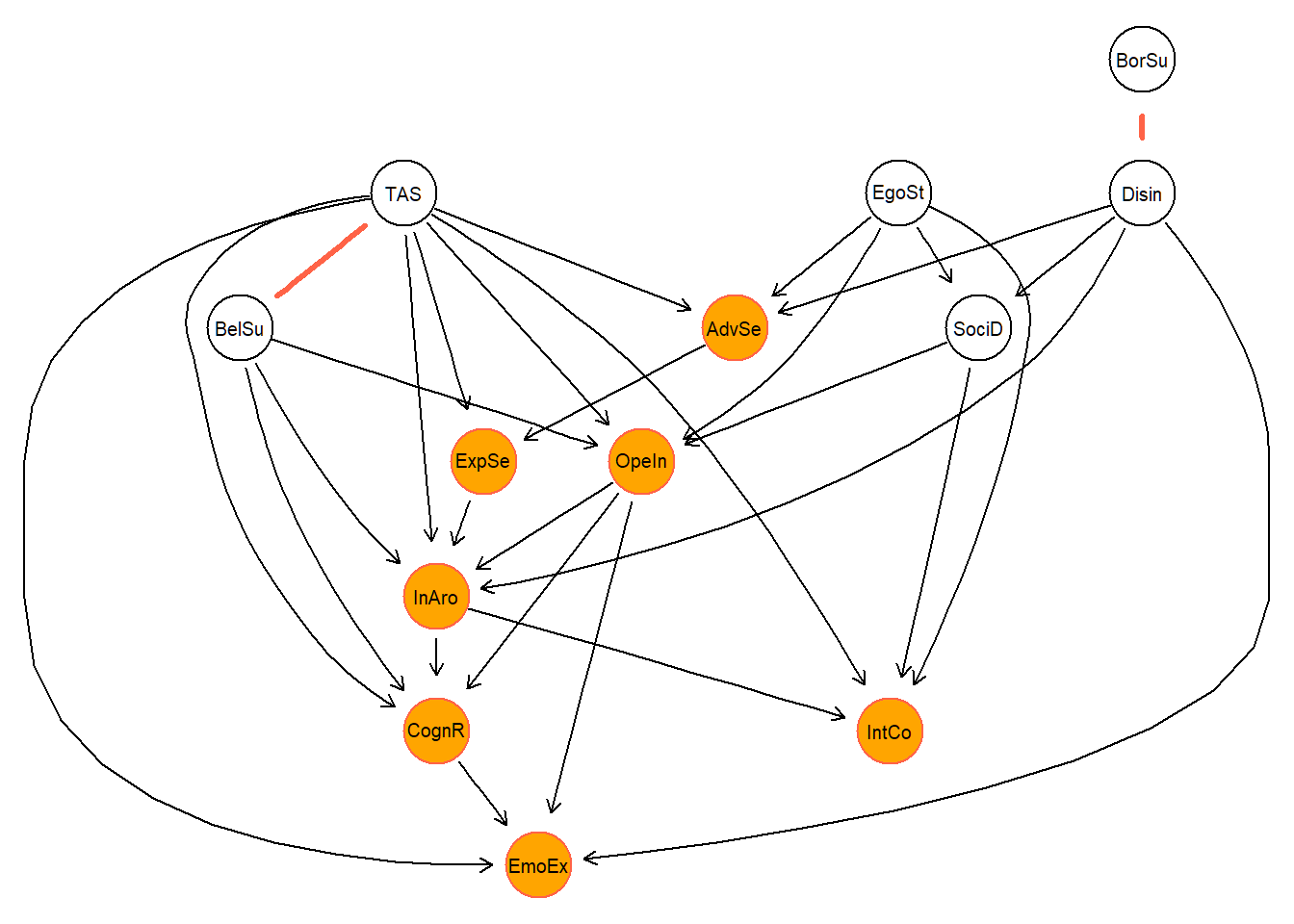
strength.plot(avgnet, astr,
  main = "Averaged network", shape = "ellipse", threshold = thresh, layout = "dot",
  highlight = list(
    nodes = c("Disin", "EgoSt", "TAS"),
    col = "tomato", fill = "orange"
  )
)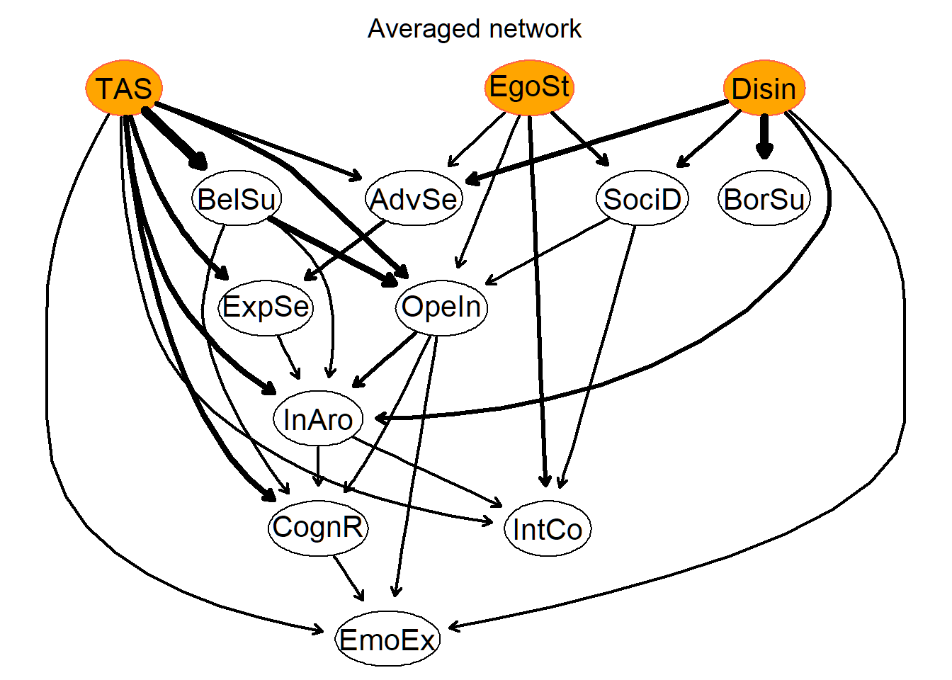
And the centrality plot of the Bayesian network, this time with outdegree and indegree as centrality measures.
centr_bn <- qgraph(avgnet, DoNotPlot = T)
centralityPlot(centr_bn, theme_bw = T, scale = "z-scores")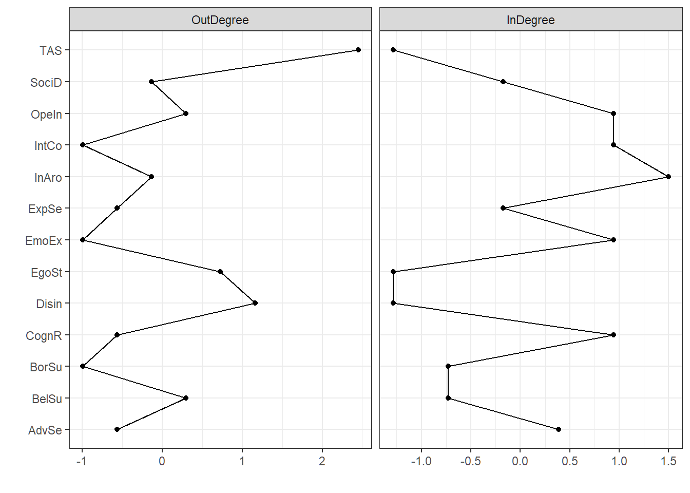
We can then learn the parameter estimates.
fitted.bn <- bnlearn::bn.fit(avgnet, rdata2, method = "mle")
# print(fitted.bn)
Let’s look at the ranking of strengths associated with the TAS…
rank <- bootnet[bootnet$from == "TAS" & bootnet$strength > 0.5, c("from", "to", "strength")]
print(rank[order(-rank$strength), ])
## from to strength
## 50 TAS ExpSe 1.00
## 53 TAS OpeIn 1.00
## 54 TAS BelSu 1.00
## 56 TAS InAro 1.00
## 59 TAS CognR 1.00
## 58 TAS IntCo 0.89
## 55 TAS EmoEx 0.69
## 49 TAS AdvSe 0.57… and at the ranking of directional probabilities associated with outgoing edges and the TAS:
rank <- bootnet[bootnet$from == "TAS" & bootnet$direction > 0.5, c("from", "to", "direction")]
print(rank[order(-rank$direction), ])
## from to direction
## 51 TAS BorSu 1.0000000
## 59 TAS CognR 0.9450000
## 56 TAS InAro 0.9300000
## 55 TAS EmoEx 0.8768116
## 58 TAS IntCo 0.8146067
## 53 TAS OpeIn 0.7600000
## 60 TAS SociD 0.7500000
## 54 TAS BelSu 0.7400000
## 57 TAS EgoSt 0.5937500
## 50 TAS ExpSe 0.5550000
## 49 TAS AdvSe 0.5438596Cross validating the BN results
predcor <- structure(numeric(13), names = c("AdvSe", "ExpSe", "BorSu", "Disin", "TAS", "OpeIn", "BelSu", "EmoEx", "InAro", "EgoSt", "IntCo", "CognR", "SociD"))

for (var in names((predcor))) {
  xval <- bn.cv(avgnet,
    data = rdata2, loss = "cor", method = "k-fold",
    loss.args = list(target = var), runs = 10
  )
  predcor[var] <- mean(sapply(xval, function(x) attr(x, "mean")))
}

round(predcor, digits = 3)
## AdvSe ExpSe BorSu Disin TAS OpeIn BelSu EmoEx InAro EgoSt IntCo CognR SociD
## 0.356 0.446 0.405 NA NA 0.633 0.563 0.458 0.631 NA 0.400 0.604 0.307summary(predcor)## Min. 1st Qu. Median Mean 3rd Qu. Max. NA's
## 0.3073 0.4014 0.4524 0.4804 0.5936 0.6327 3Using the above-derived threshold, edge strenghts are determined by direction probability
boottab <- bootnet[bootnet$strength > thresh & bootnet$direction > 0.5, ] ## edges in avgnet
nrow(boottab)
## [1] 30astr3 <- boottab ## table with direction probabilities
astr3$strength <- astr3$direction ## use the direction probabilities for edge widthLet’s also plot directionality as part of the avgnet network. Which arcs have the clearest directionality?
# Histogram of directionality as part of the avgnet network
ggplot(data = astr3, aes(x = paste0(from, "->", to), y = direction)) +
  geom_bar(stat = "identity") +
  geom_hline(yintercept = 0.50, linetype = "dashed", color = "red") +
  coord_flip() +
  theme(
    axis.text.x = element_text(angle = 90, hjust = 1),
    axis.title.x = element_blank()
  ) +
  theme_minimal() +
  labs(title = "direction probabilities of edges in network")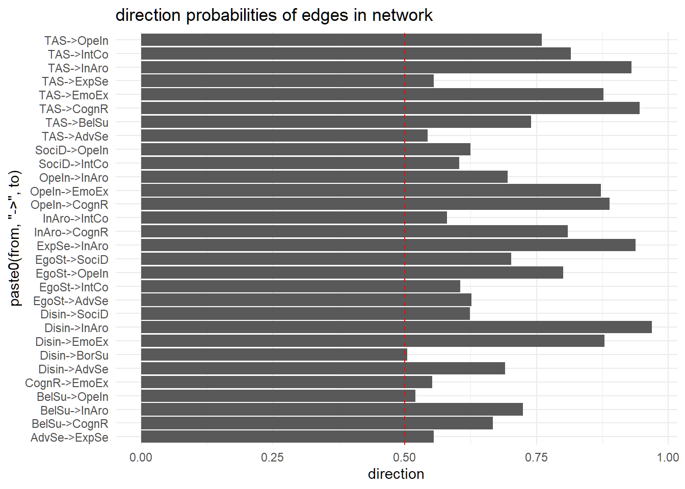
In a nutshell: The further away from the dotted red line, the more consensus there was across the bootstrapped networks regarding the direction of the edge. Vice versa, the closer to the red dotted line, the less we can be certain on the edge direction i.e., the direction could well be reversed, or alternatively, there is a mutual influence between the two nodes/ variables. In case of the TAS, we see mostly well-defined directions with absorption influencing other traits rather than the other way round.
The estimated dag is part of a so-called Complete Partially Directed Acycical Graph. A CPDAG describes the set of DAGS which are identical in terms of their score. Let’s examine the CPDAG more closely.
par(mfrow = c(1, 1))
cpdag <- cpdag(avgnet)
nrow(undirected.arcs(cpdag(cpdag)))
## [1] 4undirected.arcs(cpdag)## from to
## [1,] "BorSu" "Disin"
## [2,] "Disin" "BorSu"
## [3,] "TAS" "BelSu"
## [4,] "BelSu" "TAS"graphviz.plot(cpdag,
highlight = list(
nodes = descendants(cpdag, "TAS"), col = "tomato", fill = "orange",
arcs = undirected.arcs(cpdag), lwd = 3
)
) The cpdag shows that there are only two undirected edges, giving us further evidence of this one particular DAG. For clarity purposes; the orange nodes refer to all traits that are directly affected by the TAS. Finally, we check whether the DAG and corresponding CPDAG graph are actually valid graphs (see documentation on pcalg package.)
isValidGraph(t(amat(avgnet)), type = "dag", verbose = TRUE)## [1] TRUEisValidGraph(t(amat(cpdag)), type = "cpdag", verbose = TRUE)## [1] TRUEisValidGraph(t(amat(cpdag)), type = "pdag", verbose = TRUE)## [1] TRUEThe scenario of being highly susceptible in becoming absorbed
Absorption comes in degrees; somebody might be more susceptible in becoming absorbed than others who might remain, in general, more rational. Let’s examine the scenario of those people being very susceptible in becoming absorbed through simulation by making use of the previously estimated DAG. We do this by intervening on the TAS; we provide ‘evidence’ to the TAS by setting it hypothetically to its maximum possible value, and then examine how that subsequently affects the whole network. In other words: we
propagate evidence in the network to analyse high-absorption.
plotbn <- bn_to_graphNEL(avgnet)

# all variables are continuous
node.class <- c(
  "AdvSe" = FALSE, "ExpSe" = FALSE, "BorSu" = FALSE, "Disin" = FALSE, "TAS" = FALSE, "OpeIn" = FALSE,
  "BelSu" = FALSE, "EmoEx" = FALSE, "InAro" = FALSE,
  "EgoSt" = FALSE, "IntCo" = FALSE, "CognR" = FALSE, "SociD" = FALSE
)

tree.init.p <- Initializer(
  dag = plotbn, data = rdata2,
  node.class = node.class,
  propagate = TRUE
)

tree.init.p@propagated
## [1] TRUEtree.post <- AbsorbEvidence(tree.init.p, vars = c("TAS"), values = list(3)) # #remember, we work with standardized data
# check variables and values
tree.post@absorbed.variables## [1] "TAS"tree.post@absorbed.values## $TAS
## [1] 3div <- PlotCGBN(tree.init.p, tree.post, fontsize = 24)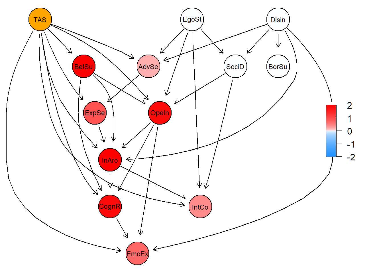
The plot shows the increase in mean activation of all nodes after propagation of ‘hard evidence’ to the TAS (orange). More red refers to being more affected due to the TAS.
For example, we can examine the impact of being highly susceptible in absorption compared to the average susceptibility in absorption, and what that implies for the susceptibility of being emotionally engaged.
varm <- "EmoEx"
marg.2 <- Marginals(tree.post, varm)
marg.1 <- Marginals(tree.init.p, varm)
mgns <- list(marg.1$marginals[[1]], marg.2$marginals[[1]])
names(mgns) <- c(varm, varm)
types <- c(marg.1$types[1], marg.2$types[1])
marg <- list(marginals = mgns, types = types)
SummaryMarginals(marg.1)
## Mean SD n
## EmoEx -0.06827712 0.9850553 1## Mean SD n
## EmoEx -0.06827712 0.9850553 1
SummaryMarginals(marg.2)## Mean SD n
## EmoEx 1.012537 0.9161935 1## Mean SD n
## EmoEx 1.012537 0.9161935 1
PlotMarginals(marg, groups = c("before", "after"))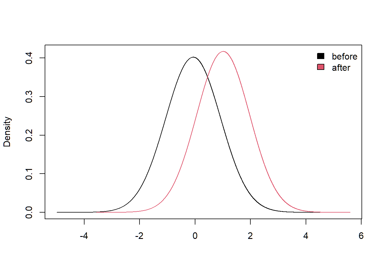
Comparing factor and network models
Finally, let’s examine the network model compared to the factor model as used in the original paper.
detach(package:bnlearn, unload = TRUE)

yvars <- colnames(R13)
ny <- length(yvars)
n_sample <- 523

# latent constructs to be measured (etas)
latents <- c(
  "Absorption permissiveness",
  "Sensation seeking",
  "Social desirability"
)

# short names
lvars <- c(
  "AP", # absorption permissiveness
  "SS", # sensation seeking
  "SD" # Social desirability
)

ne <- length(lvars)
Factor models
Based on the factor loading matrix, the three latent variables were initially indexed (measured) as follows:
lambda <- matrix(c(
  # P V W
  0, 1, 0, # Thrill and adventure seeking
  0, 1, 0, # Experience seeking
  0, 1, 0, # Boredom susceptibility
  0, 1, 0, # Disinhibition
  1, 0, 0, # TAS
  # 1, 0, 0, # Peak experiences
  # 1, 0, 0, # Dissociated experience
  1, 0, 0, # Openness to inner experiences
  1, 0, 0, # Belief in supernatural
  1, 0, 0, # Emotional extraversion
  1, 0, 0, # Intrinsic arousal
  0, 0, 1, # Ego strength
  0, 1, 1, # Intellectual control
  1, 0, 0, # Cognitive regression
  0, 0, 1 # Social desirability
),
ncol = ne,
byrow = TRUE,
dimnames = list(yvars, lvars)
)
However, unidimensionality does not hold for several measures (i.e. there are several cross-loadings). Lets correct them:
lambda_measurement <- lambda
lambda_measurement[1, 3] <- 1
lambda_measurement[2, 1] <- 1
lambda_measurement[2, 3] <- 1
lambda_measurement[6, 3] <- 1
lambda_measurement[8, 2] <- 1
lambda_measurement[13, 2] <- 1

lambda_measurement
## AP SS SD
## AdvSe 0 1 1
## ExpSe 1 1 1
## BorSu 0 1 0
## Disin 0 1 0
## TAS 1 0 0
## OpeIn 1 0 1
## BelSu 1 0 0
## EmoEx 1 1 0
## InAro 1 0 0
## EgoSt 0 0 1
## IntCo 0 1 1
## CognR 1 0 0
## SociD 0 1 1Original measurement model
Analysing the fit of the original 3 factor model based on the implied correlation matrix
measurementModel <- lvm(
  covs = (n_sample - 1) / n_sample * R13,
  lambda = lambda_measurement,
  nobs = n_sample,
  identification = "variance",
  latents = latents
)

measurementModel <- measurementModel %>% runmodel()
measurementModel %>% fit()
## Measure Value
## logl -8866.42
## unrestricted.logl -8825.56
## baseline.logl -9640.86
## nvar 13
## nobs 104
## npar 49
## df 55
## objective 10.01
## chisq 81.72
## pvalue 0.011
## baseline.chisq 1630.59
## baseline.df 91
## baseline.pvalue ~ 0
## nfi 0.95
## pnfi 0.57
## tli 0.97
## nnfi 0.97
## rfi 0.92
## ifi 0.98
## rni 0.98
## cfi 0.98
## rmsea 0.030
## rmsea.ci.lower 0.015
## rmsea.ci.upper 0.044
## rmsea.pvalue 0.99
## aic.ll 17830.85
## aic.ll2 17841.21
## aic.x -28.28
## aic.x2 179.72
## bic 18039.57
## bic2 17884.03
## ebic.25 18165.25
## ebic.5 18290.93
## ebic.75 18391.48
## ebic1 18542.30# measurementModel %>% parameters
# measurementModel %>% MIsresults_measurementModel <- measurementModel %>% runmodel()Alternative factor model: Second-order g Model
lambda_g <- cbind(lambda_measurement, g = 0)
beta_g <- cbind(matrix(0, ne + 1, ne + 1))
beta_g[1:ne, ne + 1] <- 1

gModel <- lvm(
  covs = (n_sample - 1) / n_sample * R13,
  lambda = lambda_g,
  beta = beta_g,
  sigma_zeta = "empty",
  nobs = n_sample,
  identification = "variance"
)

results_gModel <- gModel %>% runmodel()
Alternative: Bifactor model
lambda_bifactor <- cbind(lambda, g = 1)

bifactorModel <- lvm(
  covs = (n_sample - 1) / n_sample * R13,
  lambda = lambda_bifactor,
  sigma_zeta = "empty",
  nobs = n_sample,
  identification = "variance"
)

results_bifactorModel <- bifactorModel %>% runmodel()
Psychometric Network Model
saturatedModel <- ggm(
  covs = (n_sample - 1) / n_sample * R13,
  omega = "Full",
  nobs = n_sample
)

# Use 'runmodel' to compute parameters and fit measures
saturatedModel <- saturatedModel %>% runmodel()

# This initial model is saturated (df=0)
# saturatedModel

# Check parameters
# saturatedModel %>% parameters
Next, we canprune all non-significant edges.
prunedModel <- saturatedModel %>%
  prune(
    alpha = 0.01,
    recursive = TRUE,
    adjust = "fdr"
  )

# Check modification indices
prunedModel %>% MIs()
##
## Top 10 modification indices:
##
## var1 op var2 est mi pmi epc matrix row col group group_id
## EmoEx -- OpeIn 0 65.59 < 0.0001 0.26 omega 8 6 fullsample 1
## EmoEx -- TAS 0 62.50 < 0.0001 0.22 omega 8 5 fullsample 1
## EmoEx -- BelSu 0 56.07 < 0.0001 0.24 omega 8 7 fullsample 1
## CognR -- EmoEx 0 48.67 < 0.0001 0.24 omega 12 8 fullsample 1
## InAro -- EmoEx 0 41.44 < 0.0001 0.22 omega 9 8 fullsample 1
## TAS -- AdvSe 0 28.07 < 0.0001 0.15 omega 5 1 fullsample 1
## ExpSe -- AdvSe 0 27.27 < 0.0001 0.21 omega 2 1 fullsample 1
## EgoSt -- TAS 0 19.42 < 0.0001 0.15 omega 10 5 fullsample 1
## EgoSt -- ExpSe 0 19.05 < 0.0001 0.17 omega 10 2 fullsample 1
## EmoEx -- ExpSe 0 18.32 < 0.0001 0.17 omega 8 2 fullsample 1Finally, apply and compare two optimization techniques from the psychonetrics package
# Stepup estimation
prunedModel_stepup <- prunedModel %>%
  stepup()
prunedModel_stepup %>% fit() # Model fit
## Measure Value
## logl -8853.81
## unrestricted.logl -8825.56
## baseline.logl -9640.86
## nvar 13
## nobs 91
## npar 45
## df 46
## objective 9.97
## chisq 56.50
## pvalue 0.14
## baseline.chisq 1630.59
## baseline.df 78
## baseline.pvalue ~ 0
## nfi 0.97
## pnfi 0.57
## tli 0.99
## nnfi 0.99
## rfi 0.94
## ifi 0.99
## rni 0.99
## cfi 0.99
## rmsea 0.021
## rmsea.ci.lower ~ 0
## rmsea.ci.upper 0.037
## rmsea.pvalue 1.0
## aic.ll 17797.63
## aic.ll2 17806.31
## aic.x -35.50
## aic.x2 146.50
## bic 17989.31
## bic2 17846.47
## ebic.25 18104.73
## ebic.5 18220.15
## ebic.75 18312.49
## ebic1 18451.00# Modelsearch
prunedModel_modelsearch <- prunedModel %>%
modelsearch()
prunedModel_modelsearch %>% fit() # Model fit## Measure Value
## logl -8853.81
## unrestricted.logl -8825.56
## baseline.logl -9640.86
## nvar 13
## nobs 91
## npar 45
## df 46
## objective 9.97
## chisq 56.50
## pvalue 0.14
## baseline.chisq 1630.59
## baseline.df 78
## baseline.pvalue ~ 0
## nfi 0.97
## pnfi 0.57
## tli 0.99
## nnfi 0.99
## rfi 0.94
## ifi 0.99
## rni 0.99
## cfi 0.99
## rmsea 0.021
## rmsea.ci.lower ~ 0
## rmsea.ci.upper 0.037
## rmsea.pvalue 1.0
## aic.ll 17797.63
## aic.ll2 17806.31
## aic.x -35.50
## aic.x2 146.50
## bic 17989.31
## bic2 17846.47
## ebic.25 18104.73
## ebic.5 18220.15
## ebic.75 18312.49
## ebic1 18451.00Let’s compare the fit results of the network models.
compare(
  saturated = saturatedModel,
  pruned = prunedModel,
  stepup = prunedModel_stepup,
  search = prunedModel_modelsearch
)
## model DF AIC BIC RMSEA Chisq Chisq_diff DF_diff p_value
## saturated 0 17833.13 18220.75
## stepup 46 17797.63 17989.31 0.021 56.50 56.50 46 0.14
## search 46 17797.63 17989.31 0.021 56.50 ~ 0 0 < 0.0001
## pruned 58 17990.80 18131.37 0.084 273.67 217.17 12 < 0.0001
##
## Note: Chi-square difference test assumes models are nested.Plot the GGM
net1 <- getmatrix(prunedModel_modelsearch, "omega")
rownames(net1) <- colnames(net1) <- colnames(rdata2)
qgraph(net1,
layout = "spring",
title = "Pruned model with modelsearch",
palette = "colorblind",
groups = list(
"Absorption permissiveness" = which(lambda[, 1] == 1),
"Sensation seeking" = which(lambda[, 2] == 1),
"Social desirability" = which(lambda[, 3] == 1)
)
)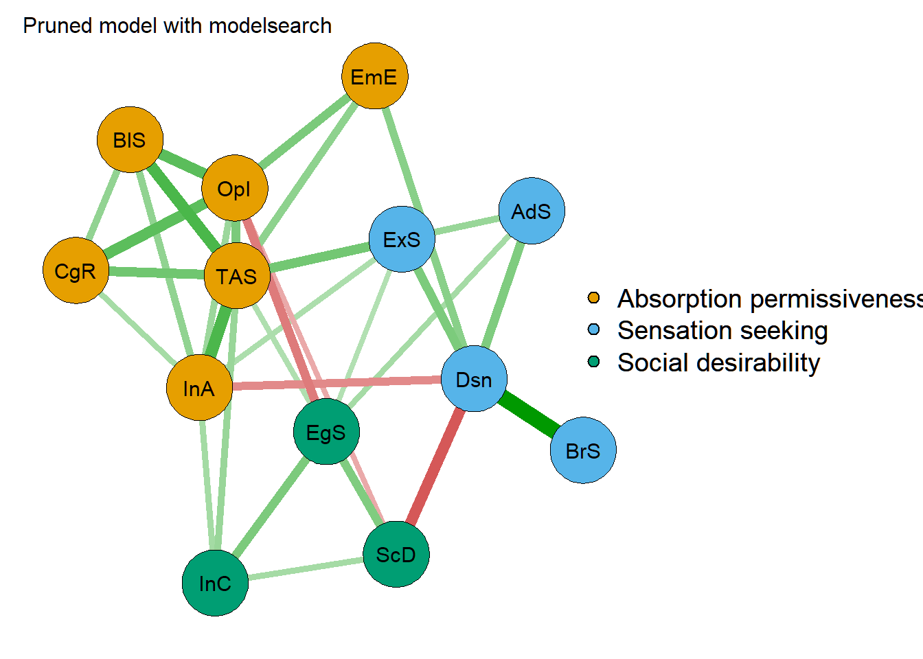 Finally, let’s compare the GGM network model (pruned and imporved with modelsearch) with the factor models:
compare(
  saturated = saturatedModel,
  ggm_modelsearch = prunedModel_modelsearch,
  measurement = results_measurementModel,
  bifactor_model = results_bifactorModel,
  gmodel = results_gModel
)
## model DF AIC BIC RMSEA Chisq Chisq_diff DF_diff p_value
## saturated 0 17833.13 18220.75
## ggm_modelsearch 46 17797.63 17989.31 0.021 56.50 56.50 46 0.14
## bifactor_model 51 17900.62 18126.38 0.059 143.50 87.00 5 < 0.0001
## measurement 55 17830.85 18039.57 0.030 81.72 61.77 4 < 0.0001
## gmodel 55 17839.74 18048.46 0.035 90.62 8.89 0 < 0.0001
##
## Note: Chi-square difference test assumes models are nested.Conclusion
Based on the comparison of fit results, we would conclude that the network model fits best to the traits data. A network interpretation of traits mutually affecting each other would then be favored over factor models. Note, however, that the above described comparison is intended to be confirmatory rather than exploratory, as was the case here. Replicating the initial study, that is collecting new data on the included traits in the orginal study, and comparing the fit of the here-found network structure with this newly-collected data would be preferable.
In any case, I hope you enjoyed following along and explore the concept of network analysis in the domain of multiple traits, and how you can do these types of complementary analyses with as little as factor loadings and a factor-intercorrelation matrix to estimate the underlying corelation matrix.
In case you have any questions, then drop me a line!
References
Kumar, V., Pekala, R. J., & Cummings, J. (1996). Trait factors, state effects, and hypnotizability. International Journal of Clinical and Experimental Hypnosis, 44(3), 232-249.
Mõttus, R. and Allerhand, M. (2017). Why do traits come together? the underlying trait and network approaches. SAGE handbook of personality and individual differences, 1:1–22.
Tellegen, A. (1981). Practicing the two disciplines for relaxation and enlightenment: Comment on “Role of the feedback signal in electromyograph biofeedback: The relevance of attention” by Qualls and Sheehan. Journal of Experimental Psychology: General, 110, 217–226. http://dx.doi.org/10.1037/0096-3445.110.2.217
Tellegen, A., & Atkinson, G. (1974). Openness to absorbing and selfaltering experiences (“absorption”), a trait related to hypnotic susceptibility. Journal of Abnormal Psychology, 83, 268–277. http://dx.doi.org/10.1037/h0036681
Tellegen, A. (1992). Note on structure and meaning of the MPQ Absorption Scale. Unpublished Manuscript, Department of Psychology, University of Minnesota.