Learning the causal structure of the optimal experience of flow during music performance
knitr::include_graphics("/img/flow_drop.jpg", error = FALSE)
Summary
In this blog, I examine the music-induced optimal state of flow using two algorithms for causal structure learning: Greedy-Equivalent-Search (GES) and the PC algorithm. Background knowledge on the preconditions of flow is incorporated to optimize the search process. For causal inference, I make use of Pearl’s do-calculus and the Intervention calculus when DAG is Absent algorithm (IDA) from the pcalg R package.
Background
Flow is a pleasurable, optimal state of mind going together with a total immersion in an activity (Chicksentmihalji, 1990). Flow has also drawn attention in music research, recognizing it as being important for optimal musical performance. In this context, Wrigley and Emmerson (2011) examined the subjective experience of flow during music performance by administering the self-report Flow State Scale-2 (FSS-2) to 236 students immediately after their musical performance. This research has led to many more studies in the music domain (Tan & Sin, 2019) but, despite this increase, it is still unclear how the dimensions of flow interact, mutually reinforce each other, and together constitute and maintain the experiential state of flow.
Question
What is the internal structure of flow during music performance?
Libraries
library(qgraph)
library(igraph)
library(bnlearn)
library(Rgraphviz)
library(tidyverse)
library(gplots)
library(plyr)
library(magrittr)
library(e1071)
library(parallel)
library(corrplot)
library(CTT)
library(networktools)
library(matrixcalc)
library(Matrix)
library(reshape2)
library(MASS)
library(lavaan)
library(lavaanPlot)
library(rcausal)
library(DOT)
library(pcalg)
library(tpc) # enables 'time-ordered data' with the pc-algorithm
library(tidySEM)
library(DiagrammeR)

## Set seed
set.seed(123)
Data
This blog continues on the study by Wrigley and Emmerson (2011) by focusing on the internal structure of flow. Let’s start by deriving the underlying correlation and covariance matrices of the data collected in the study by Wrigley and Emmerson (2011). To do this, we have to go back to the dissertation by Wrigley (2005), entitled Improving Music Performance Assessment.
Let the matrix of factor loadings be “L” and “F” the inter-factor correlation matrix. The implied correlation matrix (Σ) is then given using the following equation, with “L’” representing the transposed matrix of L:
Σ = LFL′
Let’s read in the factor loadings reported in the dissertation (on p. 142).
# first, read in factor loadings from p.142
L <- as.matrix(c(0.79, 0.65, 0.57, 0.46, 0.68, 0.85, 0.58, 0.19, 0.78))
colnames(L) <- paste0("F", 1)
rownames(L) <- paste0("V", 1:9)
Since flow is conceptualized by Wrigley (2005) as one latent factor that underlies or ‘causes’ its nine manifestations, the inter-factor correlation matrix is set to ‘1’.
F <- 1
F <- as.matrix(F)
colnames(F) <- rownames(F) <- paste0("F", 1)
Let’s derive the implied correlation matrix with the matrices above
R <- L %*% F %*% t(L)
diag(R) <- 1
mycor <- round(as.matrix(R),2)
Define the variable names and check for positive definiteness of the matrix
colnames(mycor)<-c("balance", "merging", "goals", "feedback", "concentration","control","selfawareness", "time", "autotelic")

rownames(mycor) <- colnames(mycor)

#check pd matrix
is.positive.definite(mycor)
## [1] TRUESimilarly, derive the implied covariance matrix with the additional information on the standard deviations
# means and standard deviations from Wrigley (2005), p.143
mu <- c(3.610, 3.370, 4.120, 3.780, 3.530, 3.280,3.120,3.280,3.510)
stddev <- c(.700,.740,.570,.710,.860,.750,.950,.940,.940)

covMat <- stddev %*% t(stddev) * mycor
mycov <- round(as.matrix(covMat),2)

#Define variable names
colnames(mycov) = c("balance", "merging", "goals", "feedback", "concentration","control","selfawareness", "time", "autotelic")
rownames(mycov) <- colnames(mycov)

#check pd matrix
is.positive.definite(mycov)
## [1] TRUE## Plot correlation and covariance matrices
par(mfrow=c(1,2))
corrplot(mycor, method = "color", addCoef.col = "black",
number.cex = .7, cl.pos = "n", diag=T, insig = "blank")
title(main = "Estimated correlation matrix")
corrplot(mycov, method = "color", addCoef.col = "black",
number.cex = .7, cl.pos = "n", diag=T, insig = "blank")
title(main="Estimated covariance matrix")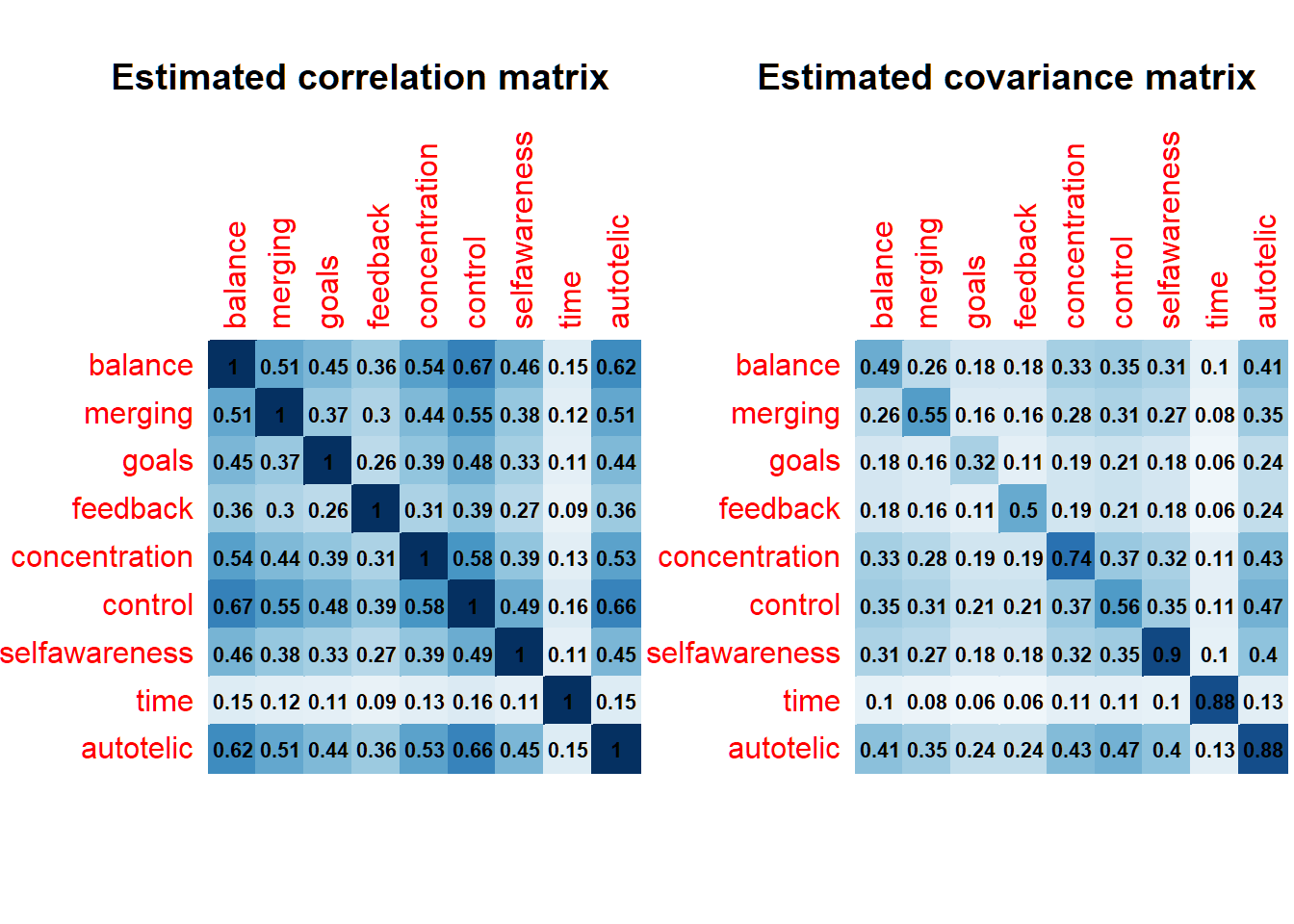
Confirmatory Factor Analysis
Let’s check the retrieved covariance matrix by, in reverse, conducting a CFA on this matrix by specifying the single-factor model of the FSS-2 as conceived by Wrigley (2005, p.142). We use the Lavaan R package.
Formulate the model, fit it, and look at the output
HS.model <- "flow = ~ balance + merging + goals + feedback + concentration + control + selfawareness + time + autotelic"

# fit the model
fit <- cfa(HS.model,
           sample.cov  = covMat,
           sample.nobs = 236)

# display summary output
summary(fit,
        standardized = TRUE,
        fit.measures=TRUE,
        rsquare = TRUE)
## lavaan 0.6-12 ended normally after 32 iterations
##
## Estimator ML
## Optimization method NLMINB
## Number of model parameters 18
##
## Number of observations 236
##
## Model Test User Model:
##
## Test statistic 0.147
## Degrees of freedom 27
## P-value (Chi-square) 1.000
##
## Model Test Baseline Model:
##
## Test statistic 746.686
## Degrees of freedom 36
## P-value 0.000
##
## User Model versus Baseline Model:
##
## Comparative Fit Index (CFI) 1.000
## Tucker-Lewis Index (TLI) 1.050
##
## Loglikelihood and Information Criteria:
##
## Loglikelihood user model (H0) -2122.525
## Loglikelihood unrestricted model (H1) -2122.451
##
## Akaike (AIC) 4281.050
## Bayesian (BIC) 4343.399
## Sample-size adjusted Bayesian (BIC) 4286.346
##
## Root Mean Square Error of Approximation:
##
## RMSEA 0.000
## 90 Percent confidence interval - lower 0.000
## 90 Percent confidence interval - upper 0.000
## P-value RMSEA <= 0.05 1.000
##
## Standardized Root Mean Square Residual:
##
## SRMR 0.002
##
## Parameter Estimates:
##
## Standard errors Standard
## Information Expected
## Information saturated (h1) model Structured
##
## Latent Variables:
## Estimate Std.Err z-value P(>|z|) Std.lv Std.all
## flow =~
## balance 1.000 0.553 0.791
## merging 0.867 0.085 10.195 0.000 0.479 0.649
## goals 0.584 0.067 8.747 0.000 0.323 0.568
## feedback 0.589 0.085 6.934 0.000 0.325 0.459
## concentration 1.058 0.098 10.787 0.000 0.585 0.681
## control 1.147 0.082 13.966 0.000 0.634 0.847
## selfawareness 0.993 0.111 8.946 0.000 0.549 0.579
## time 0.322 0.116 2.781 0.005 0.178 0.190
## autotelic 1.324 0.104 12.685 0.000 0.732 0.780
##
## Variances:
## Estimate Std.Err z-value P(>|z|) Std.lv Std.all
## .balance 0.182 0.021 8.702 0.000 0.182 0.374
## .merging 0.315 0.032 9.937 0.000 0.315 0.578
## .goals 0.219 0.021 10.262 0.000 0.219 0.678
## .feedback 0.396 0.038 10.526 0.000 0.396 0.789
## .concentration 0.394 0.040 9.759 0.000 0.394 0.536
## .control 0.158 0.021 7.594 0.000 0.158 0.283
## .selfawareness 0.597 0.058 10.224 0.000 0.597 0.665
## .time 0.848 0.078 10.816 0.000 0.848 0.964
## .autotelic 0.344 0.039 8.857 0.000 0.344 0.391
## flow 0.306 0.044 7.024 0.000 1.000 1.000
##
## R-Square:
## Estimate
## balance 0.626
## merging 0.422
## goals 0.322
## feedback 0.211
## concentration 0.464
## control 0.717
## selfawareness 0.335
## time 0.036
## autotelic 0.609# output: Latent variables: 'Estimate' are unstandardized, 'Std.all' are
# the ‘completely standardized solution’ (matching those on p.142)
# get the test statistic for the original sample
#standardizedsolution(fit)Plot the CFA model
lavaanPlot::lavaanPlot(model = fit,
           node_options = list(shape = "box", fontname = "Helvetica"),
           edge_options = list(color = "grey"),
           coefs = TRUE,
           stand = TRUE,
           stars = "latent")
“Bridges” between preconditions and experiential features of flow
From the literature, there is convergent consensus on a) flow’s preconditions and b) the core features that constitute the flow experience (see Peifer & Engeser, 2021). Let’s find the bridge nodes between the preconditions and these ‘core’ dimensions. Bridge nodes are typically the variables with cross-loadings in factor analyses, which network analysis treats as potentially the most relevant ones for understanding relations between communities.
Define the two communities
community_structure <- c('1','2','1','1','2','2','2','2','2')
is.vector(community_structure)
## [1] TRUEnetworkflow236 <- EBICglasso(mycor, n = 236,gamma = 0.5, nlambda = 100)
is.vector(community_structure) ## [1] TRUEbridge_centrality_236 <- bridge(networkflow236, communities = community_structure,
directed = FALSE)
plot(bridge_centrality_236, include=c("Bridge Expected Influence (1-step)"),
theme_bw = F, zscore = TRUE)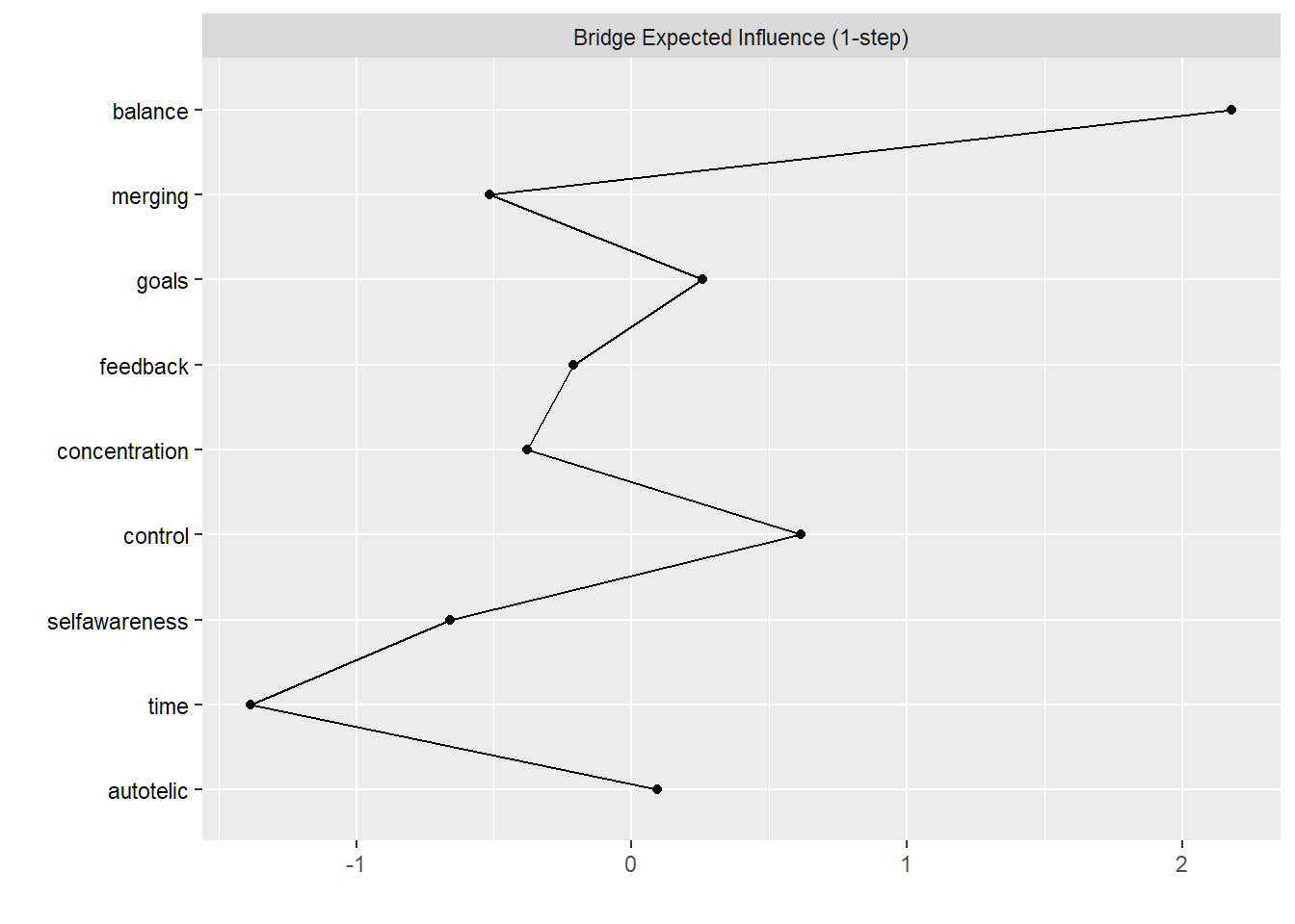
Select the top 80th percentile bridge strength.
bridge_strength_236 <- bridge_centrality_236$`Bridge Expected Influence (1-step)`

top_bridges_236 <- names(bridge_strength_236[bridge_strength_236>quantile(bridge_strength_236, probs=0.80, na.rm=TRUE)])

# Now create a new community vector where bridges are their own community
bridge_num_flow_236 <- which(names(bridge_strength_236) %in% top_bridges_236)

new_communities <- vector()

for(i in 1:length(bridge_strength_236)) {
  if(i %in% bridge_num_flow_236) {
    new_communities[i] <- "Bridge Nodes"
  } else {new_communities[i] <- community_structure[i]}
}

new_communities
## [1] "Bridge Nodes" "2" "1" "1" "2"
## [6] "Bridge Nodes" "2" "2" "2"# And now use that community vector to make groups in qgraph
qgraph(networkflow236, layout="spring",
groups = new_communities, color=c("yellow", "turquoise", "salmon"))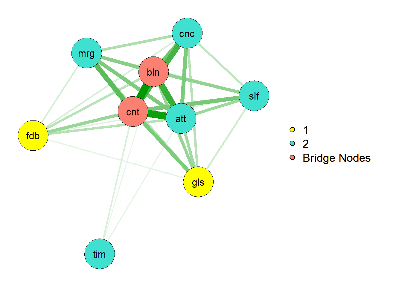
Applying the FGES algorithm with Tetrad software
Tetrad is a general causal discovery software package (see e.g., Ramsey et al., 2018). The Tetrad Runner is a R wrapper implemented for running the search algorithms from the Tetrad library in R. For more details, see the Tetrad project.
First; What is the FGES algorithm and how does it work? For a definition, we can look at its description as part of the rcausal package
tetradrunner.getAlgorithmDescription(algoId = 'fges')## FGES is an optimized and parallelized version of an algorithm developed by Meek [Meek, 1997] called the Greedy Equivalence Search (GES). The algorithm was further developed and studied by Chickering [Chickering, 2002]. GES is a Bayesian algorithm that heuristically searches the space of CBNs and returns the model with highest Bayesian score it finds. In particular, GES starts its search with the empty graph. It then performs a forward stepping search in which edges are added between nodes in order to increase the Bayesian score. This process continues until no single edge addition increases the score. Finally, it performs a backward stepping search that removes edges until no single edge removal can increase the score. More information is available here and here. The reference is Ramsey et al., 2017.
## The algorithms requires a decomposable score—that is, a score that for the entire DAG model is a sum of logged scores of each variables given its parents in the model. The algorithms can take all continuous data (using the SEM BIC score), all discrete data (using the BDeu score) or a mixture of continuous and discrete data (using the Conditional Gaussian score); these are all decomposable scores.
## It requires the score.
## It accepts the prior knowledge.In the tetrad GUI, a correlation or covariance matrix can be directly used as input for the FGES algorithm. Tetrad’s R version, however, is not yet able to use summary data. We therefore make use here of simulated data based on the covariance matrix. The here-obtained results are, however, exactly the same as when using the covariance matrix in the Tetrad GUI.
Generate simulated data based on the available summary data, with the assumption on normality
dat2 <- round(mvrnorm(n = 236, mu = mu, Sigma = covMat, empirical = T),2)

# checking the means
colMeans(dat2)
## balance merging goals feedback concentration
## 3.610085 3.369873 4.120042 3.780339 3.530297
## control selfawareness time autotelic
## 3.280297 3.120127 3.279958 3.509873# Define variable names
colnames(dat2)=c("balance", "merging", "goals", "feedback", "concentration","control","selfawareness", "time", "autotelic")
head(dat2)## balance merging goals feedback concentration control selfawareness time
## [1,] 3.07 2.61 4.28 3.15 2.19 2.85 2.52 3.53
## [2,] 3.18 3.50 3.81 3.65 3.37 3.68 2.87 3.33
## [3,] 3.41 3.73 3.92 4.58 3.43 3.22 3.52 4.05
## [4,] 4.58 3.00 4.79 4.04 5.17 3.57 2.81 4.18
## [5,] 4.08 3.24 4.03 4.00 3.91 2.35 2.45 2.40
## [6,] 3.39 2.79 3.99 4.21 2.55 2.31 3.71 3.38
## autotelic
## [1,] 2.22
## [2,] 3.53
## [3,] 4.84
## [4,] 4.07
## [5,] 3.26
## [6,] 3.80dat2 <-as.data.frame(dat2)Next, we provide the information on the preconditions ( goals, feedback, and balance) preceding the core features of flow. In addition, from ….. we assume that goals and feedback ‘cause’ balance. Our list of temporal node tiers then becomes:
temporal <- list(c("goals", "feedback"),
                 c("balance"),
                 c("merging", "concentration","control","selfawareness","time", "autotelic"))

# Define variable names
prior <- priorKnowledge(addtemporal = temporal)
## Temporal Tiers: 3
## Tier: 0
## temporal node: goals
## temporal node: feedback
## Tier: 1
## temporal node: balance
## Tier: 2
## temporal node: merging
## temporal node: concentration
## temporal node: control
## temporal node: selfawareness
## temporal node: time
## temporal node: autotelicCompute the FGES search using the following settings
tetradrunner <- tetradrunner(algoId = 'fges', #select causal algorithm
                             scoreId = 'sem-bic', #evaluation score used
                             df = dat2, # dataset
                             dataType = 'continuous', # type of data
                             #faithfulnessAssumed = TRUE,
                             maxDegree = -1,
                             priorKnowledge = prior, # add prior knowledge
                             numberResampling = 100, # bootstrapping
                             resamplingEnsemble = 2, # Majority
                             addOriginalDataset = TRUE,
                             verbose=TRUE)

tetradrunner$edges
## [1] "feedback --- goals [feedback --- goals]:0,8812;[no edge]:0,1188;"
## [2] "control --> concentration [concentration --> control]:0,0594;[concentration <-- control]:0,8416;[concentration --- control]:0,0297;[no edge]:0,0693;"
## [3] "balance --> concentration [balance --> concentration]:0,6139;[no edge]:0,3861;"
## [4] "balance --> control [balance --> control]:1,0000;"
## [5] "goals --> control [control <-- goals]:0,6832;[no edge]:0,3168;"
## [6] "goals --> balance [balance <-- goals]:1,0000;"
## [7] "control --> merging [control --> merging]:0,8416;[control <-- merging]:0,0099;[control --- merging]:0,0297;[no edge]:0,1188;"
## [8] "balance --> autotelic [autotelic <-- balance]:0,9307;[no edge]:0,0693;"
## [9] "control --> autotelic [autotelic <-- control]:0,7030;[autotelic --> control]:0,2277;[autotelic --- control]:0,0594;[no edge]:0,0099;"
## [10] "control --> selfawareness [control --> selfawareness]:0,6832;[control <-- selfawareness]:0,0297;[no edge]:0,2871;"
## [11] "feedback --> balance [balance <-- feedback]:0,9604;[no edge]:0,0396;"tetradrunner$nodes ## [1] "autotelic" "balance" "concentration" "control"
## [5] "feedback" "goals" "merging" "selfawareness"
## [9] "time"graph <- tetradrunner$graph
graph$getAttribute('BIC')
nodes <- graph$getNodes()
for(i in 0:as.integer(nodes$size()-1)){
node <- nodes$get(i)
cat(node$getName(),": ",node$getAttribute('BIC'),"\n")
}## autotelic : 161.3682
## balance : 215.7634
## concentration : 169.2742
## control : 276.794
## feedback : 165.1898
## goals : 258.5794
## merging : 170.7576
## selfawareness : 103.5411
## time : 33.18062graph_dot <- tetradrunner.tetradGraphToDot(tetradrunner$graph)
#dot(graph_dot)
#graph_dot
# reduce amount of decimal places in the initial output to 2
graph_dot2 <- strsplit(x = graph_dot,
split = "(?<=[^0-9.])(?=\\d)|(?<=\\d)(?=[^0-9.])", perl = T) %>%
unlist %>%
lapply(function(x){if(!is.na(as.numeric(x)))x<-round(as.numeric(x),2)%>%
format(nsmall=2);x}) %>%
paste(collapse="")
myGraph <- grViz(graph_dot2)
myGraphPC algorithm with the pcalg package
In addition to GES as a score-based algorithm, we also apply the PC algorithm as a conditional independence algorithm. What is the PC algorithm and how does it work?
tetradrunner.getAlgorithmDescription(algoId = 'pc-all')## PC algorithm (Spirtes and Glymour, Social Science Computer Review, 1991) is a pattern search which assumes that the underlying causal structure of the input data is acyclic, and that no two variables are caused by the same latent (unmeasured) variable. In addition, it is assumed that the input data set is either entirely continuous or entirely discrete; if the data set is continuous, it is assumed that the causal relation between any two variables is linear, and that the distribution of each variable is Normal. Finally, the sample should ideally be i.i.d.. Simulations show that PC and several of the other algorithms described here often succeed when these assumptions, needed to prove their correctness, do not strictly hold. The PC algorithm will sometimes output double headed edges. In the large sample limit, double headed edges in the output indicate that the adjacent variables have an unrecorded common cause, but PC tends to produce false positive double headed edges on small samples.
## The PC algorithm is correct whenever decision procedures for independence and conditional independence are available. The procedure conducts a sequence of independence and conditional independence tests, and efficiently builds a pattern from the results of those tests. As implemented in TETRAD, PC is intended for multinomial and approximately Normal distributions with i.i.d. data. The tests have an alpha value for rejecting the null hypothesis, which is always a hypothesis of independence or conditional independence. For continuous variables, PC uses tests of zero correlation or zero partial correlation for independence or conditional independence respectively. For discrete or categorical variables, PC uses either a chi square or a g square test of independence or conditional independence (see Causation, Prediction, and Search for details on tests). In either case, the tests require an alpha value for rejecting the null hypothesis, which can be adjusted by the user. The procedures make no adjustment for multiple testing. (For PC, CPC, JPC, JCPC, FCI, all testing searches.)
## It requires the independence test.
## It accepts the prior knowledge.Instead of tetrad, we make use of the pcalg package to showcase the features of this package and to use some of its features that are not available in Tetrad/ Rcausal package.
# define sufficient statistics
suffStat <- list(C = mycor, n = 236)

# specify tiers like we did above for FGES, based on the distinction between
# preconditions and core flow features
tiers <- c(2,3,1,1,3,3,3,3,3)

# we use code adapted from
# https://github.com/erenaldis/GaussianStructureLearning/blob/master/application.R

V <- colnames(mycor)

alphas    <- seq(0.01, 0.1, 0.01)
scores    <- c()

detach("package:bnlearn", unload = TRUE)

for (alpha in alphas) {

  ## estimate CPDAG
  tpc.fit <- tpc(suffStat  = list(C = mycor, n = 236),
                 indepTest = gaussCItest, # partial correlations
                 alpha     = alpha,
                 labels    = colnames(mycor),
                 tiers     = tiers)

  s_dag <- pdag2dag(tpc.fit@graph)$graph

  # BIC scores
  score <- new("GaussL0penObsScore", dat2)
  scores <- c(scores, score$global.score(as(s_dag, "GaussParDAG")))

  optimal.alpha <- alphas[which.max(scores)] # 0.04
}
data.frame (alphas = alphas,scores = scores) %>%
ggplot(aes(alphas, scores)) +
geom_line(color="red") +
geom_point(size = 2, color = "red") +
scale_x_continuous(limits=c(0.01,0.10), breaks=seq(0.01,0.1,0.01)) +
geom_vline(xintercept = c(0, optimal.alpha),
linetype="longdash", color = "grey65", size=0.5) +
labs(title ="BIC Score versus alpha") +
theme_minimal()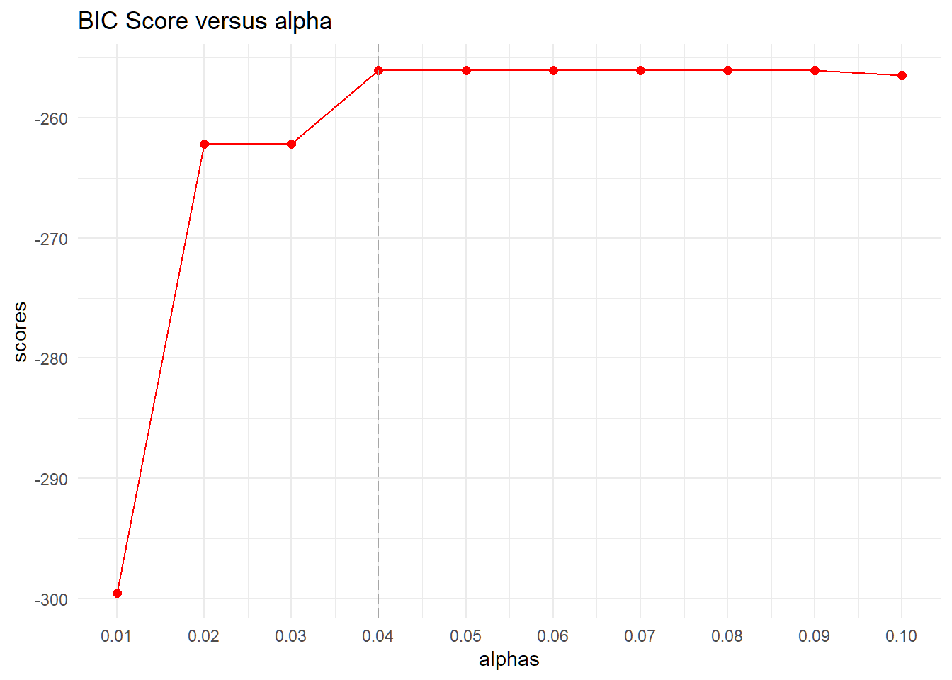
tpc.fit <- tpc(suffStat = list(C = mycor, n = 236),
              indepTest = gaussCItest,
                  alpha = optimal.alpha,
                 labels = colnames(mycor),
                  tiers = tiers)

#show estimated CPDAG
  par(mfrow=c(1,1))
  plot(tpc.fit, main = "Estimated CPDAG")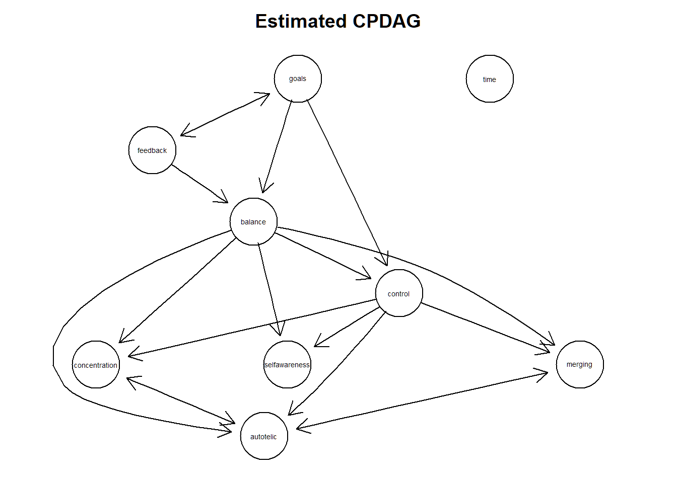
Extract the corresponding adjacency matrix “amat” of the cpdag:
adjmat <-as(tpc.fit, "amat")A valid DAG?
isValidGraph(amat = adjmat, type = "dag",verbose = T) ## [1] FALSEA valid CPDAG?
isValidGraph(amat = adjmat, type = "cpdag",verbose = T) ## [1] FALSEa valid PDAG?
isValidGraph(amat = adjmat, type = "pdag",verbose = T)## [1] TRUESo, it appears we have a maximally oriented partially directed acyclic graph, also known as maximal PDAG. this graph contains fewer undirected edges than their corresponding CPDAGs and thus contains a smaller set of equivalent fitting DAGs. This maximal PDAG arises here because of thaving imposed a partial ordering of variables (so called tiers) implicit to applying the tpc package before conducting the causal structure learning process. See also Scheines, R., Spirtes, P., Glymour, C., Meek, C., and Richardson, T. (1998).The TETRAD project: constraint based aids to causal model specification. Multivar. Behav. Res., 33 (1), 65–117.
Let’s examine in more detail how many DAGS there are left in the PDAG and how they look like.
tpc.res <- pdag2allDags(adjmat, verbose = FALSE)
tpc.res
## $dags
## [,1] [,2] [,3] [,4] [,5] [,6] [,7] [,8] [,9] [,10] [,11] [,12] [,13] [,14]
## [1,] 0 0 1 1 0 0 0 0 0 1 0 0 0 0
## [2,] 0 0 1 1 0 0 0 0 0 1 0 0 0 0
## [3,] 0 0 1 1 0 0 0 0 0 1 0 0 0 0
## [4,] 0 0 1 1 0 0 0 0 0 1 0 0 0 0
## [5,] 0 0 1 1 0 0 0 0 0 1 0 0 0 0
## [6,] 0 0 1 1 0 0 0 0 0 1 0 0 0 0
## [,15] [,16] [,17] [,18] [,19] [,20] [,21] [,22] [,23] [,24] [,25] [,26]
## [1,] 1 0 0 1 0 0 0 1 0 0 0 0
## [2,] 1 0 0 1 0 0 0 0 0 0 0 0
## [3,] 1 0 0 1 0 0 0 1 0 0 0 0
## [4,] 1 0 0 1 0 0 0 0 0 0 0 0
## [5,] 1 0 0 0 0 0 0 1 0 0 0 0
## [6,] 1 0 0 0 0 0 0 0 0 0 0 0
## [,27] [,28] [,29] [,30] [,31] [,32] [,33] [,34] [,35] [,36] [,37] [,38]
## [1,] 0 0 0 0 0 0 0 0 0 0 1 0
## [2,] 0 0 0 1 0 0 0 0 0 0 1 0
## [3,] 0 0 0 0 0 0 0 0 0 0 1 0
## [4,] 0 0 0 1 0 0 0 0 0 0 1 0
## [5,] 0 0 0 0 0 0 0 0 0 0 1 0
## [6,] 0 0 0 1 0 0 0 0 0 0 1 0
## [,39] [,40] [,41] [,42] [,43] [,44] [,45] [,46] [,47] [,48] [,49] [,50]
## [1,] 0 0 0 1 0 0 1 1 0 1 0 0
## [2,] 0 0 0 1 0 0 1 1 0 1 0 0
## [3,] 0 0 0 1 0 0 0 1 0 1 0 0
## [4,] 0 0 0 1 0 0 0 1 0 1 0 0
## [5,] 0 0 0 1 0 0 1 1 0 1 0 0
## [6,] 0 0 0 1 0 0 1 1 0 1 0 0
## [,51] [,52] [,53] [,54] [,55] [,56] [,57] [,58] [,59] [,60] [,61] [,62]
## [1,] 0 0 0 0 1 0 0 0 0 1 0 0
## [2,] 0 0 0 0 1 0 0 0 0 1 0 0
## [3,] 0 0 0 0 1 0 0 0 0 1 0 0
## [4,] 0 0 0 0 1 0 0 0 0 1 0 0
## [5,] 0 0 0 0 1 0 0 0 0 1 0 0
## [6,] 0 0 0 0 1 0 0 0 0 1 0 0
## [,63] [,64] [,65] [,66] [,67] [,68] [,69] [,70] [,71] [,72] [,73] [,74]
## [1,] 0 0 0 0 0 0 0 0 0 0 1 0
## [2,] 0 0 0 0 0 0 0 0 0 0 1 0
## [3,] 0 0 0 0 0 0 0 0 0 0 1 0
## [4,] 0 0 0 0 0 0 0 0 0 0 1 0
## [5,] 0 0 0 0 0 0 0 0 0 0 1 1
## [6,] 0 0 0 0 0 0 0 0 0 0 1 1
## [,75] [,76] [,77] [,78] [,79] [,80] [,81]
## [1,] 0 0 0 1 0 0 0
## [2,] 0 0 0 1 0 0 0
## [3,] 0 0 1 1 0 0 0
## [4,] 0 0 1 1 0 0 0
## [5,] 0 0 0 1 0 0 0
## [6,] 0 0 0 1 0 0 0
##
## $nodeNms
## [1] "balance" "merging" "goals" "feedback"
## [5] "concentration" "control" "selfawareness" "time"
## [9] "autotelic"# Plot function (see pcald documentation)
plotAllCPs2 <- function(tpc.res) {
require(graph)
p <- sqrt(ncol(tpc.res$dags))
nDags <- ceiling(sqrt(nrow(tpc.res$dags)))
par(mfrow = c(nDags, nDags))
for (i in 1:nrow(tpc.res$dags)) {
amat <- matrix(tpc.res$dags[i,],p,p, byrow = TRUE)
colnames(amat) <- rownames(amat) <- tpc.res$nodeNms
plot(as(amat, "graphNEL"))
}
}
par(mfrow = c(3,3))
plotAllCPs2(tpc.res)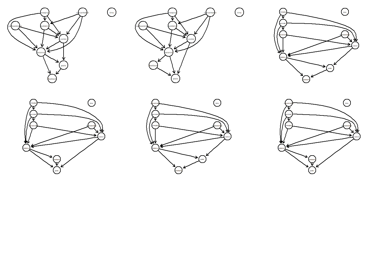
To sum up: we have tpcfitgraph as a valid PDAG, whose equivalence class consists of in total six DAGs. This plot allows us evaluate the relationships between variables. In other words, combining the PC algorithm together with the information on the temporal ordering of preconditions and core features of flow, we end up with 6 potential DAGs that are identical in terms of fit.
Intervention calculus when DAG is Absent: IDA
However, we do not yet know how strong the causal relationships are. To do so, we make use of Pearl’s do-calculus and the Intervention calculus when DAG is Absent algorithm (IDA) from the pcalg package. Ida estimates the multiset of possible joint total causal effects of variables (X) onto variables (Y) from observational data via adjustment.
# adapted from https://github.com/btaschler/scl_replicate/tree/b4ddeddf715d26254e75f4798e4a375539cee89b/R

run_ida <- function(X, sig_level, skel.method) {

  G_hat           <- matrix(nrow = ncol(X), ncol = ncol(X))
  dimnames(G_hat) <- list(colnames(X), colnames(X))

  suffStat <- list(C = cor(X), n = nrow(X))

  pc.fit <- tpc::tpc(suffStat,
                     indepTest   = gaussCItest,
                     alpha       = sig_level,
                     p           = ncol(suffStat$C),
                     tiers       = tiers)

  covX <- cov(X)

  for (j in 1:ncol(X)){

# Idafast estimates the multiset of possible total causal effects of one variable -x- on several target variables -y- from observational data
    eff <- pcalg::idaFast(j, 1:ncol(X), covX, pc.fit@graph)

# https://www.datasciencemadesimple.com/row-wise-minimum-row-minimum-in-dataframe-r-2/
    # rowMins returns minimum value of each row of the matrix.
    G_hat[j,] <- matrixStats::rowMins( abs(eff) )
    }

  Output <- list( g_hat = G_hat )

  return(Output)
}

idamatrix <- run_ida(dat2, 0.05, "stable")
we can plot the IDA values together with the PDAG using the igraph R package.
#weight matrix
idamatrix <- round(as.matrix(idamatrix[["g_hat"]]),2)

W <- idamatrix
W[ which(W == 0) ] <-  .Machine$double.xmin
W[ which(W == 0) ] <- 0.001
Convert our PDAG graph into igraph format via bn-format
G <- bnlearn::as.bn(tpc.fit@graph)
G <- bnlearn::as.igraph(G)

G2 <-  graph_from_adjacency_matrix(as.matrix(W) *
       as.matrix(get.adjacency(G, type="both")),
        mode="directed", weighted=TRUE)

E(G2)[ which(E(G2)$weight == .Machine$double.xmin) ]$weight <-  0.0

plot.igraph(G2,
            edge.label=E(G2)$weight,
            edge.arrow.size = 0.5,
            layout=layout_in_circle, rescale=T)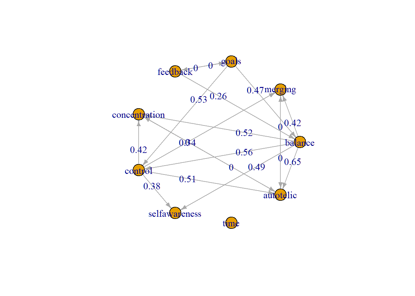
Alternatively, we can plot the IDA values together with the PDAG with the bnlearn package. Again, given the PDAG, note that these are the minimum values from the IDA matrix that represent the minimal causal effects when taking int account all 6 potential, equivalent DAGS.
# convert matrix W (idamatrix) to dataframe suitable for bn
# rows    -> from
# columns -> to

g <- graph.adjacency(W, weighted = TRUE)

# values in a data frame with 3 columns: from,to,value
df <- get.data.frame(g)
df$weight <- round(df$weight,3)

# bn/ cpdag
G <- bnlearn::as.bn(tpc.fit@graph)
library(bnlearn)
detach("package:tidySEM", unload=TRUE)Let’s plot it with the following function:
plot_s <- function(x,y){

  # convert arc to edge
  mat <- matrix(0,length(nodes(x)),length(nodes(x)))
  rownames(mat) <- nodes(x)
  colnames(mat) <- nodes(x)

  for (i in 1:dim(arcs(x))[1]){
    mat[nodes(x)==arcs(x)[i,1],nodes(x)==arcs(x)[i,2]]<-1
  }

  # create the graphAM object from the bn object
  g1 <- graphAM(adjMat = mat, edgemode = "directed")

  to.score   <- apply(y[,1:2], 1, paste, collapse = "~")
  lab        <- as.character(y[,3])
  names(lab) <- to.score

  g1 <- layoutGraph(g1, edgeAttrs=list(label=lab))

  graph.par(list(nodes = list(lwd=1,
                              lty=1,
                              fontsize=22,
                              shape="ellipse"),

                 edges = list(fontsize=10,
                              textCol="black")
                 )
            )

  nodeRenderInfo(g1) <- list(shape="ellipse")
  renderGraph(g1)
}

par(mfrow = c(1,1))
plot_s(G,df)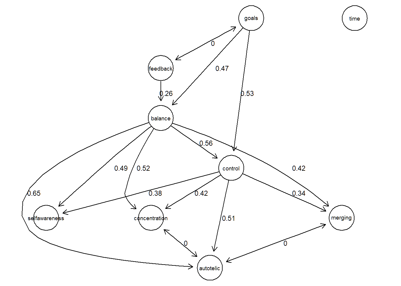
Additionally, we can bootstrap this analysis and get a notion on the directional probabilities of the estimated network.
Bootstraps <- lapply(1:100, function(x) {

  bootstrapped_model <- tpc(suffStat  = list(
    C = cor(dat2[sample(1:nrow(dat2), nrow(dat2), TRUE), ]),
    n = 236),

    indepTest = gaussCItest,
    alpha     = optimal.alpha,
    labels    = V,
    tiers     = tiers,
    verbose   = FALSE)

  return(bootstrapped_model)
})

# Are individual edges included (y/n)?
resBoots_temp <- lapply(Bootstraps, function(x)
                 ifelse(wgtMatrix(x) > 0, 1, 0))

# over all 100 bootstrap iterations, how often (%) is a particular edge included?
strength <- apply(simplify2array(resBoots_temp), 1:2, mean)

# convert matrix to dataframe for plotting
str_g       <- graph.adjacency(strength, weighted=TRUE)
strength_df <- get.data.frame(str_g)
colnames(strength_df) <- c("from","to","direction probability")

par(mfrow = c(1,1))
plot_s(G,strength_df)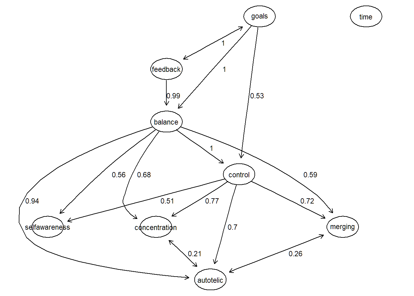
Comparing graphs of fges and pc algorithms
Finally, after having used the FGES and PC algorithms to learn the causal structure of flow, let’s compare their structures for correspondences and differences. In its essence, this follows the common procedure to use multiple learning algorithms to obtain a more robust structure.
To recap: we have the following two structures learned with the FGES and PC algorithms. Note that both contain undirected and directed edges.
Let’s make sure that both network structures are stored as objects of class bn.
# PC as bn object
bn_pc <- as.bn(tpc.fit@graph)

#FGES as bn object
nodes <-  c("balance", "merging", "goals", "feedback", "concentration","control","selfawareness", "time", "autotelic")

bn_fges <-empty.graph(nodes)

arc.set <- matrix(c(
"autotelic","merging",
"balance","concentration",
"balance","control",
"goals","control",
"balance","autotelic",
"control","selfawareness",
"feedback", "goals", # undirected
"goals", "feedback", # undirected
"control","concentration",
"autotelic","selfawareness",
"goals","balance",
"control","merging",
"control","autotelic",
"feedback","balance"),
ncol = 2, byrow = TRUE,
dimnames = list(NULL, c("from", "to")))

arcs(bn_fges) <- arc.set

# plot two graphs
#par(mfrow = c(1,1))
#graphviz.plot(bn_pc)
#graphviz.plot(bn_fges)
The SHD metric implements the Structural Hamming Distance, counting how many arcs differ between the CPDAGs of the two networks.
# the true positive (tp) arcs appear in both structures
bnlearn::compare(bn_pc, bn_fges, arcs = TRUE)
## $tp
## from to
## [1,] "balance" "concentration"
## [2,] "balance" "control"
## [3,] "balance" "autotelic"
## [4,] "goals" "balance"
## [5,] "goals" "control"
## [6,] "feedback" "balance"
## [7,] "control" "merging"
## [8,] "control" "concentration"
## [9,] "control" "selfawareness"
## [10,] "control" "autotelic"
## [11,] "goals" "feedback"
## [12,] "feedback" "goals"
##
## $fp
## from to
## [1,] "autotelic" "merging"
## [2,] "autotelic" "selfawareness"
##
## $fn
## from to
## [1,] "balance" "merging"
## [2,] "balance" "selfawareness"
## [3,] "merging" "autotelic"
## [4,] "concentration" "autotelic"
## [5,] "autotelic" "merging"
## [6,] "autotelic" "concentration"# 4 edges differ between the CPDAGs of the two network
shd(bn_pc, bn_fges) ## [1] 4Let’s compare them visually by plotting them side by side and highlight differences with colours.
par(mfrow = c(2,1))
graphviz.compare(bn_pc, bn_fges,
                 shape = "circle", layout = "dot",
                 main = c("PC", "FGES"),
                 sub = paste("SHD =", c("0", shd(bn_pc, bn_fges))),
                 diff.args = list(tp.lwd = 2, tp.col = "green"))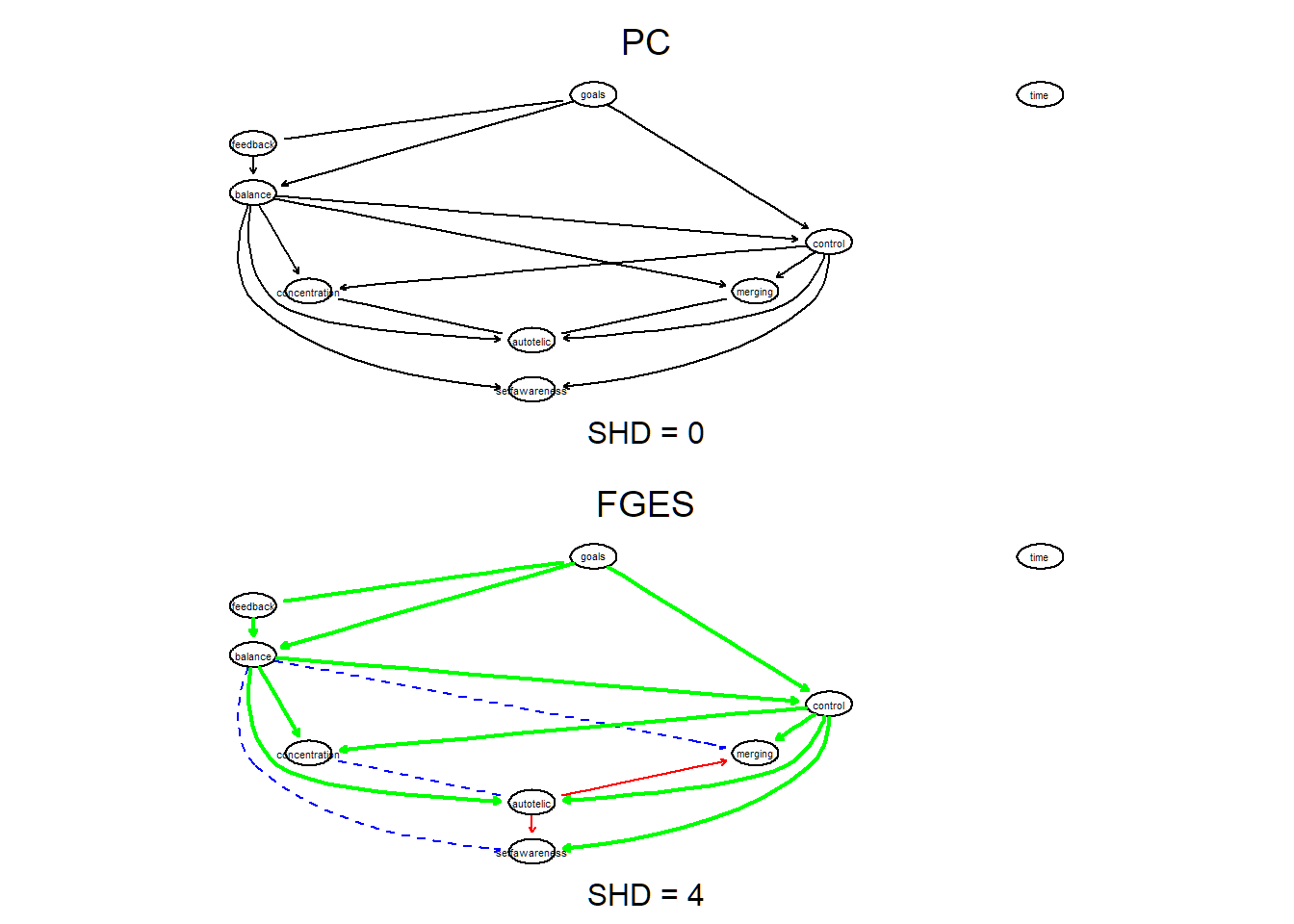
Conclusion
In this blog, I showcased how to apply two structure learning algorithms to examine the internal structure of the flow experience during music performance. Tetrad, pcalg and bnlearn are some of the most-widely used toolkits for structure learning. I showed how to apply them, and also to examine how strong the causal relationships are with the IDA algorithm.
An important takeaway is that, together with some (expert) background knowledge on the structure, these algorithms can quickly reduce the initially large set of DAGS to a potential few (in case of the PC algorithm, there were only 6 DAGS, together forming a maximum PDAG). With expert knowledge, and in case of looking explicitly for one ’best ’DAG only, this data-driven procedure can further help in discovering and explaining the mechanisms of flow.
References
Csikszentmihalyi, M. (1990). Flow: The psychology of optimal experience. New York, NY: Harper & Row.
Peifer, C. & Engeser, S. (Eds). (2021). Advances in Flow Research, 2nd Edn, (New York, NY: Springer). doi: 10.1007/978-3-030-53468-4_16
Ramsey, J.D. et al.(2018). TETRAD—A toolbox for causal discovery. In 8th International Workshop on Climate Informatics (CI 2018)
Wrigley, W.J.(2005). Improving Music Performance Assessment. PhD Doctorate Thesis. https://doi.org/10.25904/1912/332, Download here:
Wrigley, W.J. & Emmerson, S.B. (2011). The experience of the flow state in live music performance, Psychology of Music, 41, pp. 292-305, 10.1177/0305735611425903
Tan, L., & Sin, H. X. (2019). Flow research in music contexts: A systematic literature review, Musicae Scientiae doi:10.1177/1029864919877564