The phenomenology of hypnosis: A meta-analytic structural equation modeling approach
knitr::include_graphics("/img/watch.jpg", error = FALSE)
Summary
In this blog, I test an experiential model of hypnosis using a meta-analytic structural equation modeling approach (MASEM). With Bayesian network structure learning, I use a data-driven technique to examine how the initial model as proposed by Rainville and Price (2003), when slightly restructured, can be further improved.
Background
During my PhD and postdoc centered around the theme of music-induced absorption, I regularly came across the related subject of hypnosis. In this blog I want to explore this exciting subject in more detail.
In contrast to music, hypnosis is centered on the response to a usually verbal induction procedure by a clinician/experimenter that can, after following more specific suggestions, elicit changes in ideomotor, perceptual, cognitive, or emotional features and often leads to corresponding changes in subjective experience and observable behavior (Kihlstrom, 2008; Nash & Barnier, 2008). It is as a form of effortless, absorbed awareness with a present-moment focus in which imagination is often prominent (Thompson, Waeld, Tisza & Spiegel, 2016) and encouraged by suggestions, often identified by a sense of automaticity (i.e., feeling of loss of control) and reduced self-orientation (Rainville & Price, 2003).
To better understand the mechanisms that ‘drive’ hypnosis, Rainville and Price (2003) proposed an experiential model of hypnosis’ subjective experience build around the following dimensions which, when taken together, particularly characterize the feeling of being hypnotized:
1. Feeling relaxed with no arousal at all.
2. Absorbed attention while being engaged in the hypnotic process.
3. A relative absence of self-monitoring/ self-awareness.
4. An alteration in experience marked by a loss in the perception of time and place.
5. Feelings of automaticity, effortlessness or sense of loss in volitional control.
Lastly, the authors assumed that the loss in volitional control and alterations in experience were the main contributors in
6. the self-perceived depth of the hypnotic experience.
Specifically, the experiential model of hypnosis looks like this:
knitr::include_graphics("/img/modelhyp.jpg", error = FALSE)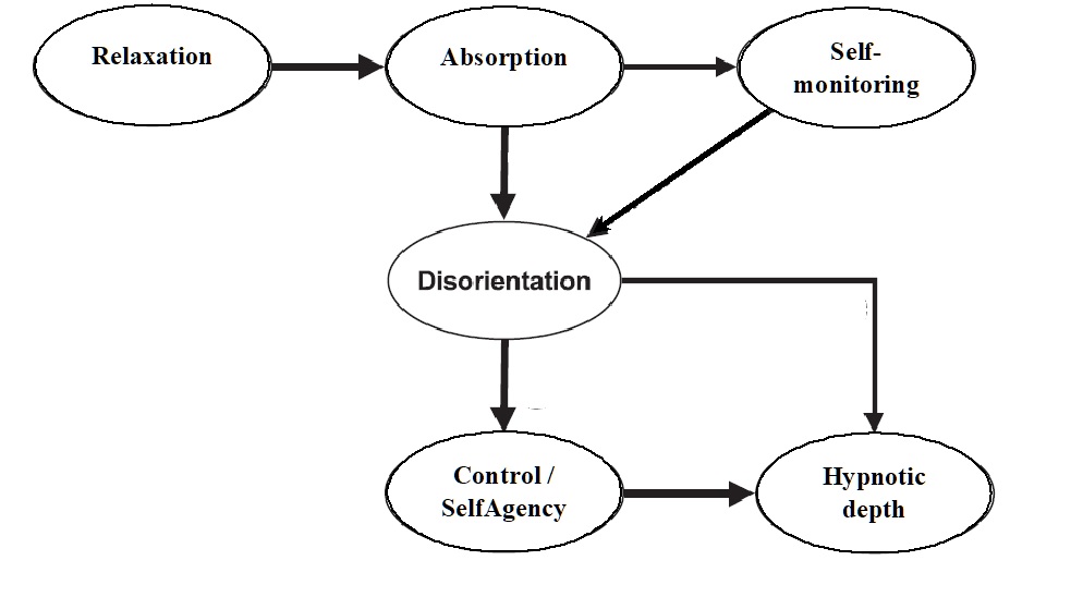
The authors further remark that, “In this model, functional interactions are proposed in which changes in distinct experiential dimensions precede changes in other dimension following the sequence of arrows” (…) where “these successive interactions need not reflect a strict temporal sequence but rather indicate a general functional interaction” (p.112). In other words, the model represents the hypothesized conditional independences between the main dimensions of hypnotic experience.
Except for the authors themselves, and despite the fact that the article is almost 20 years old, this model has never been tested thoroughly. This blog will therefore takes up this challenge.
Question
Do data on the subjective experience of being hypnotized fit the experiential model of hypnosis as originally formulated by Rainville and Price? How can a data-driven approach help further in identifying and adopting an alternative, better fitting but equally plausible model?
Method
To tackle this question we integrate Structural equation modeling (SEM) and meta-analysis (MA), combining research findings from several independent studies conducted in the past on the phenomenology of hypnosis. This combination is known as meta-analytic structural equation modeling (MASEM), a relatively new area of research used for testing hypothesized models like the model outlined above based on multiple studies.
SEM tests several a-priori formulated relations between a set of variables simultaneously. With the help of a number of fit indices, we can evaluate the fit of the model to the data. This data does not have to be raw data perse; correlation (or covariance) matrices can also be used directly as input. For more information on MASEM, see Cheung (2014;2015a;2015b) or Jak (2015).
Ok, Let’s get started!
Libraries
library(metaSEM)
library(OpenMx)
library(ggplot2)
library(ggridges)
library(tidyverse)
library(semPlot)
library(qgraph)
library(igraph)
library(corrplot)
library(bnlearn)
library(Rgraphviz)
library(SEset)
library(kableExtra)
library(tidyr)
library(ggridges)

## Set seed
set.seed(123)
Data
I’ve put the file with the correlation matrices on my osf account to access and load the correlation matrices.
# read 7 correlation matrices from 7 different hypnosis studies
cordat6X6 <- readFullMat(file = "https://osf.io/vtgf6/download",skip = 1)

# Sample sizes of the individual studies on hypnotic experiences
N <- c(173,246,241,266,565,615,523) # N = 2629
Check positive definiteness of each correlation matrix
is.pd(cordat6X6, check.aCov=FALSE, cor.analysis=TRUE, tol=1e-06)## 1 2 3 4 5 6 7
## TRUE TRUE TRUE TRUE TRUE TRUE TRUESome background information on the individual studies:
df_studies <- data.frame (
  Authors = c("Kumar & Pekala", "Pekala, Forbes and Contrisciani", "Loi", "Varga, Józsa & Kekecs","Kolto", "Terhune & Cardeña", "Kumar,Pekala & Cummings"),
  Year = c(1988, 1989, 2011, 2014, 2015, 2010, 1996),
  Sample = c(173,246,241,266,565,615,523),
  Participants =c("students","students","students","volunteers","mainly students","volunteers","students"),
  Induction = c("HGSHS", "HGSHS", "a 10-minute trance induction audio file","SHSS-A", "HGSHS:A", "WSGC","HGSHS:A"),
  Administration = c("group", "group", "individual", "individual","group","group","group")
                  )

knitr::kable(df_studies, format="html")| Authors | Year | Sample | Participants | Induction | Administration |
|---|---|---|---|---|---|
| Kumar & Pekala | 1988 | 173 | students | HGSHS | group |
| Pekala, Forbes and Contrisciani | 1989 | 246 | students | HGSHS | group |
| Loi | 2011 | 241 | students | a 10-minute trance induction audio file | individual |
| Varga, Józsa & Kekecs | 2014 | 266 | volunteers | SHSS-A | individual |
| Kolto | 2015 | 565 | mainly students | HGSHS:A | group |
| Terhune & Cardeña | 2010 | 615 | volunteers | WSGC | group |
| Kumar,Pekala & Cummings | 1996 | 523 | students | HGSHS:A | group |
Random effects analysis
A random-effects two-stage structural equation modeling (TSSEM) approach was used to conduct the MASEM analysis Cheung (2014, 2015a).
First, the correlation matrices are being combined with a random-effects model. the resulting averaged correlation matrix and the variance component of the heterogeneity variances were estimated with FIML (full information maximum likelihood estimation).
Second, we fit the structural equation model as implied by the figure depicted above on the averaged correlation matrix togehter with its asymptotic sampling covariance matrix using the weighted least square estimation method.
Stage 1 random
Since there are relatively few data (i.e., we have only 7 studies), the structure of the variance component of the random effects is restricted by specifying RE.type = “Diag”.
stage1random_6 <- tssem1(Cov = cordat6X6,
                         n = N,
                         method = "REM",
                         RE.type="Diag")
Try again if optimal conditions are not found. Note that the OpenMx status1 has to be “0” or “1”
if (stage1random_6$mx.fit$output$status$code > 1)
{ stage1random_6 <- metaSEM::rerun(stage1random_6, checkHess=F, extraTries=30, silent=TRUE)}
##
Beginning initial fit attempt
Fit attempt 0, fit=-278.588502765187, new current best! (was -278.586348601983)
Final run, for Hessian and/or standard errors and/or confidence intervals
summary(stage1random_6)##
## Call:
## meta(y = ES, v = acovR, RE.constraints = Diag(paste0(RE.startvalues,
## "*Tau2_", 1:no.es, "_", 1:no.es)), RE.lbound = RE.lbound,
## I2 = I2, model.name = model.name, suppressWarnings = TRUE,
## silent = silent, run = run)
##
## 95% confidence intervals: z statistic approximation (robust=FALSE)
## Coefficients:
## Estimate Std.Error lbound ubound z value Pr(>|z|)
## Intercept1 -5.9382e-01 1.6718e-02 -6.2658e-01 -5.6105e-01 -35.5201 < 2.2e-16
## Intercept2 6.2715e-01 1.7963e-02 5.9194e-01 6.6236e-01 34.9131 < 2.2e-16
## Intercept3 1.7087e-01 1.8742e-02 1.3413e-01 2.0760e-01 9.1170 < 2.2e-16
## Intercept4 -5.4240e-01 2.5475e-02 -5.9233e-01 -4.9247e-01 -21.2918 < 2.2e-16
## Intercept5 -2.8043e-01 1.8075e-02 -3.1585e-01 -2.4500e-01 -15.5142 < 2.2e-16
## Intercept6 -5.8408e-01 2.4439e-02 -6.3198e-01 -5.3618e-01 -23.8995 < 2.2e-16
## Intercept7 -2.0423e-01 1.8283e-02 -2.4006e-01 -1.6839e-01 -11.1703 < 2.2e-16
## Intercept8 6.8405e-01 3.1237e-02 6.2283e-01 7.4527e-01 21.8989 < 2.2e-16
## Intercept9 4.1068e-01 2.8829e-02 3.5417e-01 4.6718e-01 14.2451 < 2.2e-16
## Intercept10 1.8121e-01 2.1958e-02 1.3817e-01 2.2424e-01 8.2524 2.220e-16
## Intercept11 -4.9618e-01 2.6977e-02 -5.4905e-01 -4.4330e-01 -18.3927 < 2.2e-16
## Intercept12 -3.1377e-01 1.6455e-02 -3.4602e-01 -2.8152e-01 -19.0687 < 2.2e-16
## Intercept13 -1.4211e-01 1.9109e-02 -1.7957e-01 -1.0466e-01 -7.4368 1.033e-13
## Intercept14 -3.7542e-01 3.8175e-02 -4.5024e-01 -3.0060e-01 -9.8344 < 2.2e-16
## Intercept15 3.3169e-01 3.7273e-02 2.5864e-01 4.0474e-01 8.8989 < 2.2e-16
## Tau2_1_1 7.5583e-04 1.0413e-03 -1.2852e-03 2.7968e-03 0.7258 0.4679
## Tau2_2_2 1.1629e-03 1.1736e-03 -1.1373e-03 3.4631e-03 0.9909 0.3217
## Tau2_3_3 1.0003e-10 NA NA NA NA NA
## Tau2_4_4 3.0675e-03 2.0972e-03 -1.0429e-03 7.1780e-03 1.4627 0.1436
## Tau2_5_5 1.0001e-10 5.1269e-04 -1.0049e-03 1.0049e-03 0.0000 1.0000
## Tau2_6_6 2.8947e-03 2.1232e-03 -1.2666e-03 7.0560e-03 1.3634 0.1728
## Tau2_7_7 1.0002e-10 NA NA NA NA NA
## Tau2_8_8 5.8964e-03 3.5380e-03 -1.0380e-03 1.2831e-02 1.6666 0.0956
## Tau2_9_9 3.8002e-03 9.7130e-04 1.8965e-03 5.7039e-03 3.9125 9.135e-05
## Tau2_10_10 7.3190e-04 9.1366e-04 -1.0588e-03 2.5226e-03 0.8011 0.4231
## Tau2_11_11 3.3894e-03 2.6133e-03 -1.7326e-03 8.5114e-03 1.2970 0.1946
## Tau2_12_12 1.0002e-10 NA NA NA NA NA
## Tau2_13_13 1.0002e-10 1.0632e-03 -2.0839e-03 2.0839e-03 0.0000 1.0000
## Tau2_14_14 7.8639e-03 4.9665e-03 -1.8703e-03 1.7598e-02 1.5834 0.1133
## Tau2_15_15 7.3744e-03 5.0366e-03 -2.4971e-03 1.7246e-02 1.4642 0.1431
##
## Intercept1 ***
## Intercept2 ***
## Intercept3 ***
## Intercept4 ***
## Intercept5 ***
## Intercept6 ***
## Intercept7 ***
## Intercept8 ***
## Intercept9 ***
## Intercept10 ***
## Intercept11 ***
## Intercept12 ***
## Intercept13 ***
## Intercept14 ***
## Intercept15 ***
## Tau2_1_1
## Tau2_2_2
## Tau2_3_3
## Tau2_4_4
## Tau2_5_5
## Tau2_6_6
## Tau2_7_7
## Tau2_8_8 .
## Tau2_9_9 ***
## Tau2_10_10
## Tau2_11_11
## Tau2_12_12
## Tau2_13_13
## Tau2_14_14
## Tau2_15_15
## ---
## Signif. codes: 0 '***' 0.001 '**' 0.01 '*' 0.05 '.' 0.1 ' ' 1
##
## Q statistic on the homogeneity of effect sizes: 339.8164
## Degrees of freedom of the Q statistic: 90
## P value of the Q statistic: 0
##
## Heterogeneity indices (based on the estimated Tau2):
## Estimate
## Intercept1: I2 (Q statistic) 0.3967
## Intercept2: I2 (Q statistic) 0.5389
## Intercept3: I2 (Q statistic) 0.0000
## Intercept4: I2 (Q statistic) 0.6935
## Intercept5: I2 (Q statistic) 0.0000
## Intercept6: I2 (Q statistic) 0.7085
## Intercept7: I2 (Q statistic) 0.0000
## Intercept8: I2 (Q statistic) 0.8774
## Intercept9: I2 (Q statistic) 0.6649
## Intercept10: I2 (Q statistic) 0.2206
## Intercept11: I2 (Q statistic) 0.6836
## Intercept12: I2 (Q statistic) 0.0000
## Intercept13: I2 (Q statistic) 0.0000
## Intercept14: I2 (Q statistic) 0.7908
## Intercept15: I2 (Q statistic) 0.7712
##
## Number of studies (or clusters): 7
## Number of observed statistics: 135
## Number of estimated parameters: 30
## Degrees of freedom: 105
## -2 log likelihood: -278.5885
## OpenMx status1: 0 ("0" or "1": The optimization is considered fine.
## Other values may indicate problems.)The results show that the Q statistic is significant (Q(df=90) = 339.82, p < .05), suggesting that there is significant heterogeneity in the correlation matrices.
The I2 (representing the heterogeneity of the correlation coefficients) of the 15 correlation coefficients varies between .00 and .0.88, with several being quite high, suggesting that for these coefficients a considerable part of the variance is due to the study level.
- Intercept: The averaged correlation coefficients
- Tau2: The estimated study level variances of the correlation coefficients The pooled correlation coefficients (fixed effects)…
coef(stage1random_6, select="fixed")## Intercept1 Intercept2 Intercept3 Intercept4 Intercept5 Intercept6
## -0.5938153 0.6271501 0.1708677 -0.5423996 -0.2804268 -0.5840801
## Intercept7 Intercept8 Intercept9 Intercept10 Intercept11 Intercept12
## -0.2042259 0.6840516 0.4106775 0.1812066 -0.4961778 -0.3137690
## Intercept13 Intercept14 Intercept15
## -0.1421115 -0.3754225 0.3316909and the the variance components (the random effects)
coef(stage1random_6, select="random")## Tau2_1_1 Tau2_2_2 Tau2_3_3 Tau2_4_4 Tau2_5_5 Tau2_6_6
## 7.558289e-04 1.162888e-03 1.000307e-10 3.067521e-03 1.000119e-10 2.894669e-03
## Tau2_7_7 Tau2_8_8 Tau2_9_9 Tau2_10_10 Tau2_11_11 Tau2_12_12
## 1.000230e-10 5.896413e-03 3.800187e-03 7.319021e-04 3.389381e-03 1.000209e-10
## Tau2_13_13 Tau2_14_14 Tau2_15_15
## 1.000199e-10 7.863940e-03 7.374399e-03Extract the estimated average correlation matrix, with diagonal of the matrix filled with 1’s. Select the fixed effects and convert it into a correlation matrix
pooled6 <- vec2symMat(coef(stage1random_6,
                           select = "fixed"),
                           diag   = FALSE )

rownames(pooled6) <- colnames(pooled6) <- c("SA","AA","VC","AR","AE","AB")

pooled6 <- round(pooled6,3)

corpcor::is.positive.definite(pooled6, tol=1e-8)
## [1] TRUEThe averaged pooled correlation matrix based on the random effects model looks like this:
corrplot(pooled6, method = "color", addCoef.col = "black",
number.cex = .5, cl.pos = "n", diag=T,insig = "blank")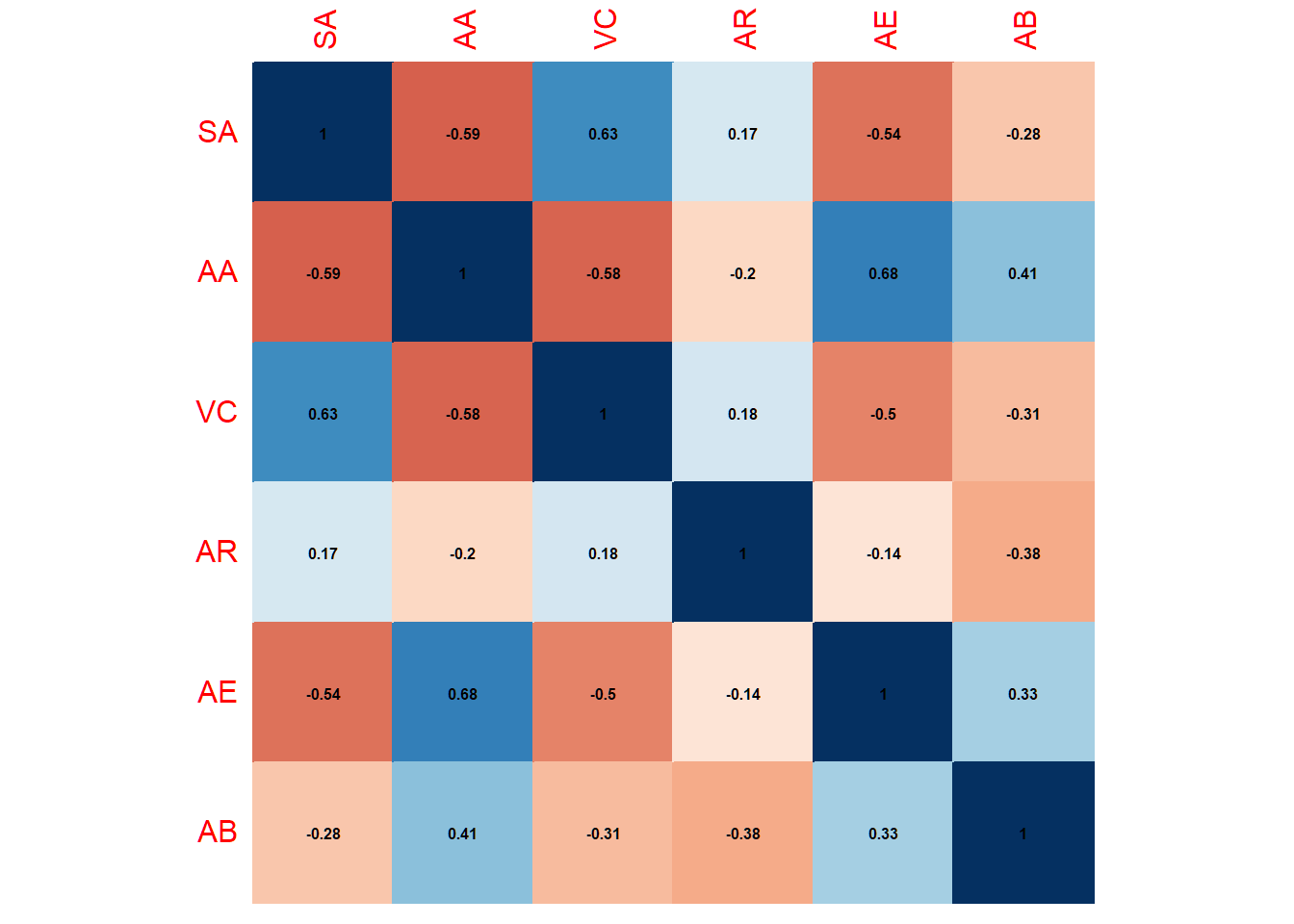 Next, we formulate the structural model to which we are going to fit the pooled correlation matrix to. To this end, we use Reticular Action Modeling (RAM) syntax, although it is also possible to use lavaan syntax first, which can the be automatically converted to RAM. Note that, since we use only observed variables and no latent variables, we only need the following two matrices A and S (explained below).
First, matrix A specifies all regression coefficients in the model:
A <- create.mxMatrix(c(0, 0, 0,0, 0,"0.1*AB2SA",
                       0, 0, "0.1*VC2AA",0, "0.1*AE2AA", 0,
                       "0.1*SA2VC",0, 0, 0,"0.1*AE2VC", 0,
                       0,0,0,0,0,0,
                       "0.1*SA2AE",0,0,0,0,"0.1*AB2AE",
                       0,0,0,"0.1*AR2AB",0,0),

                     type="Full", byrow=TRUE, ncol=6, nrow=6, name="A")
Inspect the model
dimnames(A)[[1]] <- dimnames(A)[[2]] <- c("SA","AA","VC","AR","AE","AB")
A
## FullMatrix 'A'
##
## $labels
## SA AA VC AR AE AB
## SA NA NA NA NA NA "AB2SA"
## AA NA NA "VC2AA" NA "AE2AA" NA
## VC "SA2VC" NA NA NA "AE2VC" NA
## AR NA NA NA NA NA NA
## AE "SA2AE" NA NA NA NA "AB2AE"
## AB NA NA NA "AR2AB" NA NA
##
## $values
## SA AA VC AR AE AB
## SA 0.0 0 0.0 0.0 0.0 0.1
## AA 0.0 0 0.1 0.0 0.1 0.0
## VC 0.1 0 0.0 0.0 0.1 0.0
## AR 0.0 0 0.0 0.0 0.0 0.0
## AE 0.1 0 0.0 0.0 0.0 0.1
## AB 0.0 0 0.0 0.1 0.0 0.0
##
## $free
## SA AA VC AR AE AB
## SA FALSE FALSE FALSE FALSE FALSE TRUE
## AA FALSE FALSE TRUE FALSE TRUE FALSE
## VC TRUE FALSE FALSE FALSE TRUE FALSE
## AR FALSE FALSE FALSE FALSE FALSE FALSE
## AE TRUE FALSE FALSE FALSE FALSE TRUE
## AB FALSE FALSE FALSE TRUE FALSE FALSE
##
## $lbound: No lower bounds assigned.
##
## $ubound: No upper bounds assigned.Matrix S specifies all variances and covariances in the model:
S <- create.mxMatrix(c("0.1*var_SA",
                       0, "0.1*var_AA",
                       0, 0, "0.1*var_VC",
                       0, 0, 0, 1,
                       0, 0, 0, 0, "0.1*var_AE",
                       0, 0, 0, 0, 0, "0.1*var_AB"),
                     byrow=TRUE, type="Symm", ncol=6, nrow=6, name="S")

# inspect the model
dimnames(S)[[1]] <- dimnames(S)[[2]] <- c("SA","AA","VC","AR","AE","AB")
S
## SymmMatrix 'S'
##
## $labels
## SA AA VC AR AE AB
## SA "var_SA" NA NA NA NA NA
## AA NA "var_AA" NA NA NA NA
## VC NA NA "var_VC" NA NA NA
## AR NA NA NA NA NA NA
## AE NA NA NA NA "var_AE" NA
## AB NA NA NA NA NA "var_AB"
##
## $values
## SA AA VC AR AE AB
## SA 0.1 0.0 0.0 0 0.0 0.0
## AA 0.0 0.1 0.0 0 0.0 0.0
## VC 0.0 0.0 0.1 0 0.0 0.0
## AR 0.0 0.0 0.0 1 0.0 0.0
## AE 0.0 0.0 0.0 0 0.1 0.0
## AB 0.0 0.0 0.0 0 0.0 0.1
##
## $free
## SA AA VC AR AE AB
## SA TRUE FALSE FALSE FALSE FALSE FALSE
## AA FALSE TRUE FALSE FALSE FALSE FALSE
## VC FALSE FALSE TRUE FALSE FALSE FALSE
## AR FALSE FALSE FALSE FALSE FALSE FALSE
## AE FALSE FALSE FALSE FALSE TRUE FALSE
## AB FALSE FALSE FALSE FALSE FALSE TRUE
##
## $lbound: No lower bounds assigned.
##
## $ubound: No upper bounds assigned.Stage 2
stage2random_6 <- tssem2(stage1random_6,
                         Amatrix = A,
                         Smatrix = S,
                         diag.constraints = F,
                         intervals="LB",
                         model.name = "TSSEM2 Random Effects Analysis Phenomenology of hypnosis")
Try again if optimal conditions are not found
if (stage2random_6$mx.fit$output$status$code > 1)
{ stage2random_6 <- metaSEM::rerun(stage2random_6, checkHess=F, extraTries=100, silent=TRUE)}summary(stage2random_6)##
## Call:
## wls(Cov = pooledS, aCov = aCov, n = tssem1.obj$total.n, RAM = RAM,
## Amatrix = Amatrix, Smatrix = Smatrix, Fmatrix = Fmatrix,
## diag.constraints = diag.constraints, cor.analysis = cor.analysis,
## intervals.type = intervals.type, mx.algebras = mx.algebras,
## model.name = model.name, suppressWarnings = suppressWarnings,
## silent = silent, run = run)
##
## 95% confidence intervals: Likelihood-based statistic
## Coefficients:
## Estimate Std.Error lbound ubound z value Pr(>|z|)
## AE2AA 0.68838 NA 0.60060 0.77875 NA NA
## VC2AA -0.24448 NA -0.33436 -0.14761 NA NA
## AR2AB -0.38220 NA -0.44402 -0.32098 NA NA
## AB2AE 0.30312 NA 0.25141 0.35512 NA NA
## SA2AE -0.50119 NA -0.55085 -0.45040 NA NA
## AB2SA -0.29342 NA -0.33047 -0.25634 NA NA
## AE2VC -0.27819 NA -0.34947 -0.20914 NA NA
## SA2VC 0.48804 NA 0.41378 0.55755 NA NA
##
## Goodness-of-fit indices:
## Value
## Sample size 2629.0000
## Chi-square of target model 115.4095
## DF of target model 7.0000
## p value of target model 0.0000
## Number of constraints imposed on "Smatrix" 0.0000
## DF manually adjusted 0.0000
## Chi-square of independence model 2896.7519
## DF of independence model 15.0000
## RMSEA 0.0768
## RMSEA lower 95% CI 0.0648
## RMSEA upper 95% CI 0.0894
## SRMR 0.0649
## TLI 0.9194
## CFI 0.9624
## AIC 101.4095
## BIC 60.2890
## OpenMx status1: 0 ("0" or "1": The optimization is considered fine.
## Other values indicate problems.)The χ2 of the hypothesized experiential model for hypnosis is significant (χ2 (2) = 115.41, p < .05) suggesting we don’t have an exact fit between the data and the model. However, the RMSEA of 0.077 suggests approximate fit, while the CFI of 0.96 indicates acceptable/good fit of the model.
The parameter estimates are all significantly different from zero, since zero is not within each of the 95% confidence intervals.
Next, let’s first check whether the parameters are correctly labelled by displaying the model graphically (i.e., plot the model with labels):
my.plot2 <- meta2semPlot(stage2random_6,
                         manNames = c("SA","AA","VC","AR","AE","AB") )

Labels <- c(
  "Self-awareness",             #SA
  "Altered state of awareness", #AA
  "Volitional control",         #VC
  "Arousal",                    #AR
  "Altered experience",         #AE
  "Inward directed absorption") #AB

mm <- matrix(c("AR"   , "AB",  "SA",
                NA    , "AE"  , NA,
                NA    , "VC", "AA"), byrow = TRUE, 3, 3)

semPaths(my.plot2, whatLabels="path", nCharEdges=10, nCharNodes=10, layout=mm, color="yellow", edge.label.cex=0.8)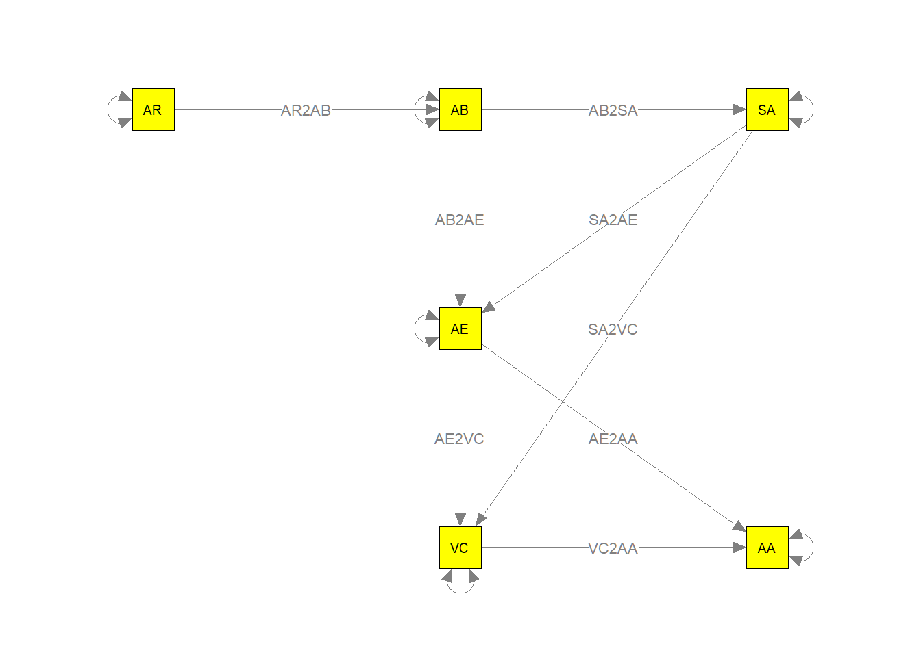
Next, let’s also plot the parameter estimates:
semPaths(my.plot2, whatLabels="est", nCharEdges=10, nCharNodes=10,layout=mm, color="green", edge.label.cex=0.8,
         nodeNames=Labels,legend.cex = 0.3)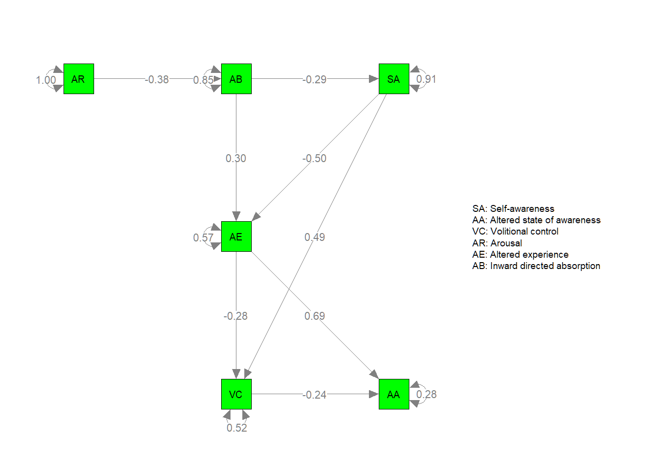
In sum, although the model overall appears to fit the data reasonably well, there appears to be room for further model inprovement.
Statistical Equivalence-Set
First, let’s take a look at the controllability values (R2 indices) of each variable to get a hunge on where a variable is best postioned in the directe network.
estimate <- EBICglasso(pooled6, n = 2106,threshold = TRUE, returnAllResults = TRUE)

# qgraph method estimates a non-symmetric omega matrix, but uses forceSymmetric to create
# a symmetric matrix (see qgraph:::EBICglassoCore line 65)
library(Matrix)

# returns the precision matrix
omega <- as.matrix(forceSymmetric(estimate$optwi))

library(qgraph)
parcor <- qgraph::wi2net(omega)
pnet <- qgraph(parcor, repulsion = .8,vsize = c(10,15), theme = "colorblind", fade = F)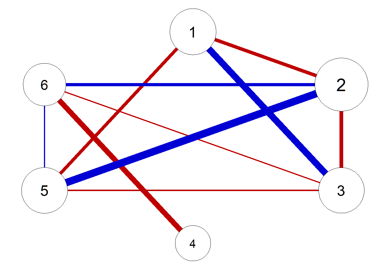
# Name the variables
dimnames(omega) <- dimnames(pooled6)
varnames <- rownames(omega)

# Estimate SE-set with rounding
SE_h <- network_to_SEset(omega, digits = 2, rm_duplicates = TRUE)
# Directed edge frequency
propd <- propcal(SE_h, rm_duplicate = TRUE, directed = TRUE)
# Plot as a network
qgraph(propd, edge.color = "darkgreen", layout = pnet$layout, edge.labels = T, maximum = 1)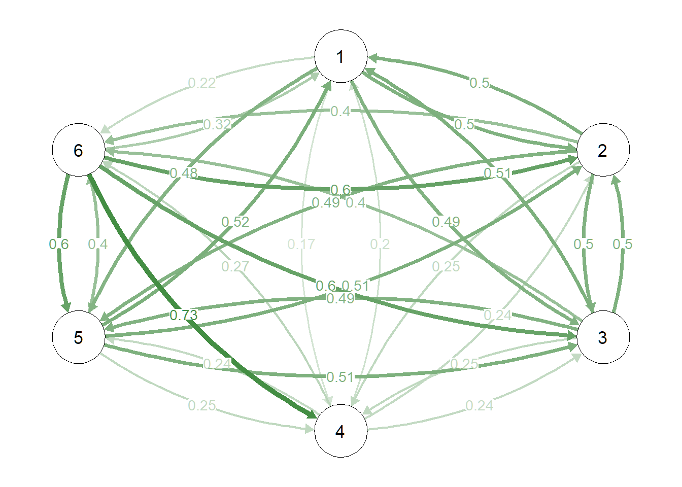
r2set <- r2_distribution(SE_h, cormat = pooled6, names = NULL, indices = c(1,2,3,4,5,6))
df <- as.data.frame(r2set, col.names = paste0("X",1:6))
df2 <- tidyr::gather(df)
p <- ggplot(df2, aes(y = key, x = value)) +
geom_density_ridges(fill = "light seagreen") +
labs(y = "Variable", x = expression(paste("Controllability value ", R^2)))
p + theme(text = element_text(size = 20),
axis.title.x = element_text(size = 20),
axis.title.y = element_text(size = 20),
panel.background = element_blank())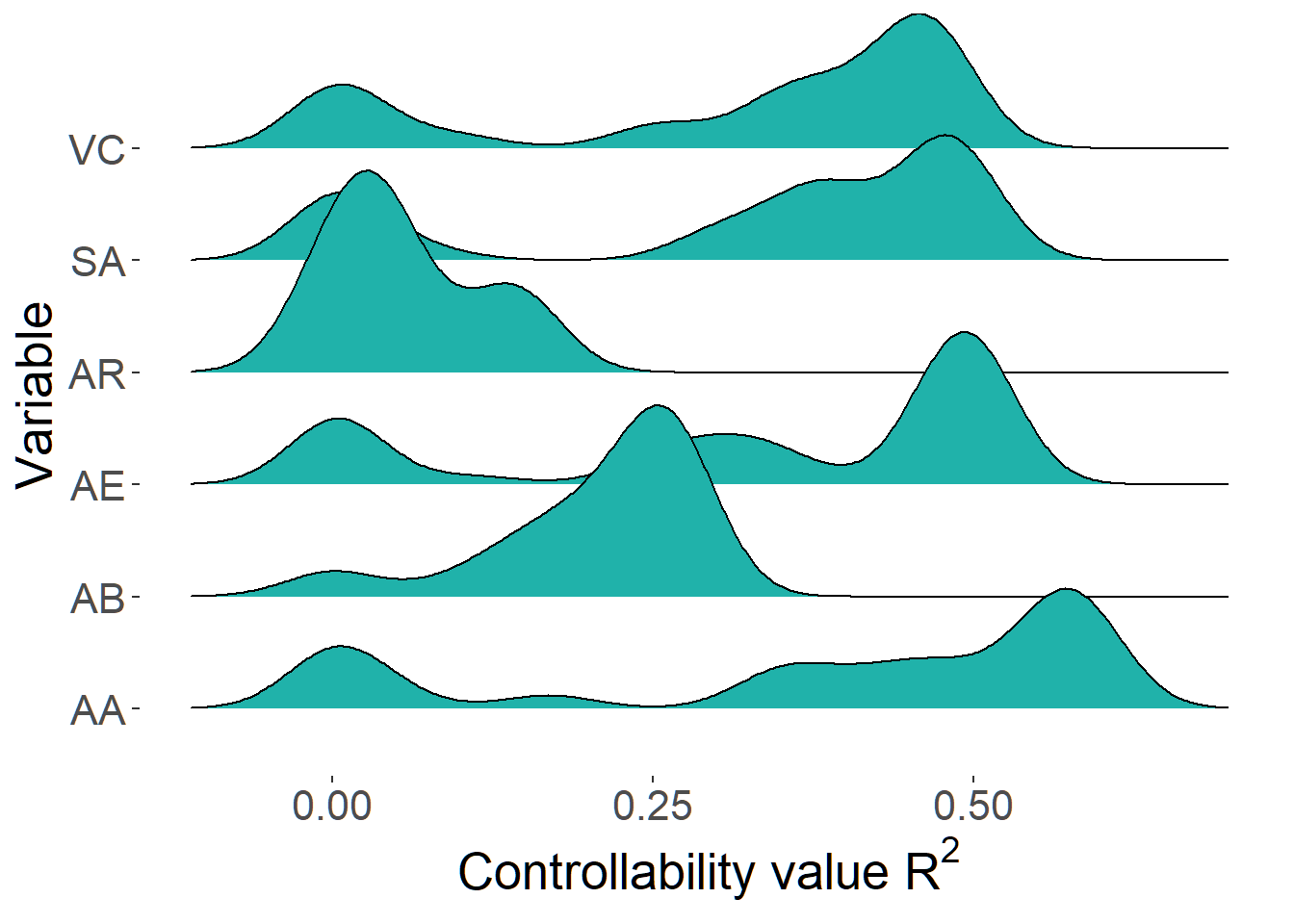 This plot shows that AR (i.e. arousal) has a relatively low controllability value. The more or less single peak of AR on the left suggests that the multiple potential directed graphs (DAGS) are consistent in the location of AR in the graph (i.e. as a starting point in the graph).
Simulating data
Next, let’s continue with applying structure learning algorithms. To do so, we need to simulate data as the algorithms used here (from the bnlearn package) only accept raw, tabular data and not correlational data.
One way to simulate data from the correlation matrix is through Cholesky decomposition. Since our goal is to obtain simulated raw data that reproduces the correlation matrix as closely as possible, we need to identify the seed with which the difference can be minimized.
minvalue <- 50
minseed <- 9000

for(i in 35000:40000) {
  set.seed(i)
  M <- chol(pooled6)
  r <- t(M) %*% matrix(rnorm(6*2629), nrow = 6, ncol = 2629)
  r <- t(r)

  rdata <-  as.data.frame(r)
  corrdata <- round(cor(rdata),3)

  diff <- abs(pooled6-corrdata)
  diff2 <- diff > 0.05

  sumdiff <- sum(diff2)

  # updating minimal value
  minvalue <- ifelse ((sumdiff < minvalue), sumdiff, minvalue)
  minseed <- ifelse ((sumdiff <= minvalue), i, minseed)
}
The values are:
minvalue## [1] 0minseed## [1] 40000The results above suggested that with setting the seed at 40000, we simulate data with which we reproduce the correlation matrix as closely as possible with only 0 coefficients that differ more than 0.05.
set.seed(minseed)

M <- chol(pooled6)
nvars <-dim(M)[1]

# number of observations to simulate
nobs <- 2629

# Random variables that follow the R correlation matrix
r <- t(M) %*% matrix(rnorm(nvars*nobs), nrow=nvars, ncol=nobs)
r <- t(r)
rdata <-  as.data.frame(r)
rrdata <- round(cor(rdata),3)

diff <- abs(pooled6-rrdata)
diff2 <- diff > 0.05
sum(diff2)
## [1] 0Let’s plot the absolute differences:
corrplot::corrplot(abs(pooled6-rrdata), method = "color", addCoef.col = "black", number.cex = .6, cl.pos = "n", diag=T, insig = "blank")
title(main="Absolute Difference")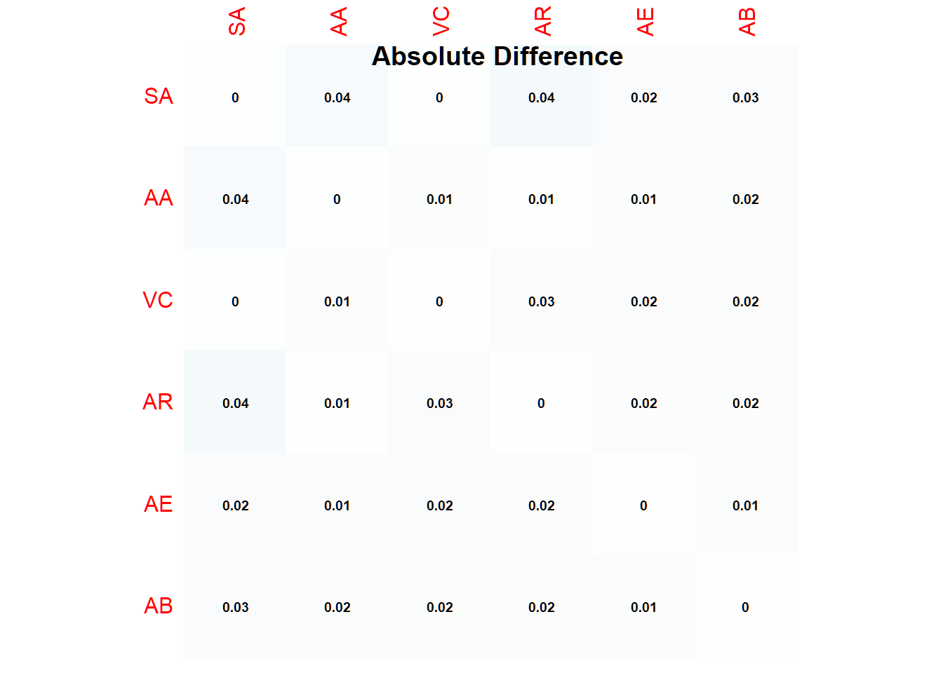
Learning the structure with multiple algorithms
Let’s source four R-functions adapted from the supplements to the 2016 article Bayesian Networks in Survey data: Robustness and Sensitivity Issues by Cugnata, Kenett & Salini.
These functions can also be found in my github account hypnosis
source("SBN_robustNet.R")
source("importance.R")
source("plot_s.R")
source("plot_DWI.R")
Next, we specify the blacklist. We forbid any outgoing edges away from AA because it is taken here to be the end- or target node:
datiBN <- rdata
nomi   <- c("SA","AA","VC","AR","AE","AB")

blacklist <-  data.frame (from = c(rep("AA",6)),
                          to   = c(colnames(datiBN)[1:6]))

# view blacklist
blacklist
## from to
## 1 AA SA
## 2 AA AA
## 3 AA VC
## 4 AA AR
## 5 AA AE
## 6 AA AB# Specify the highlight node
target_node <- "AA"Retrieve the Bayesian network structure with the most robust arcs according to different structure learning algorithms. The code was adapted from the original code by
- changing hybrid algorithms mmhc with aic and bic for mmhc without score
- constraint-based mmpc (Max-Min Parents & Children)
net <- SBN_robustNet(datiBN, blacklist = blacklist)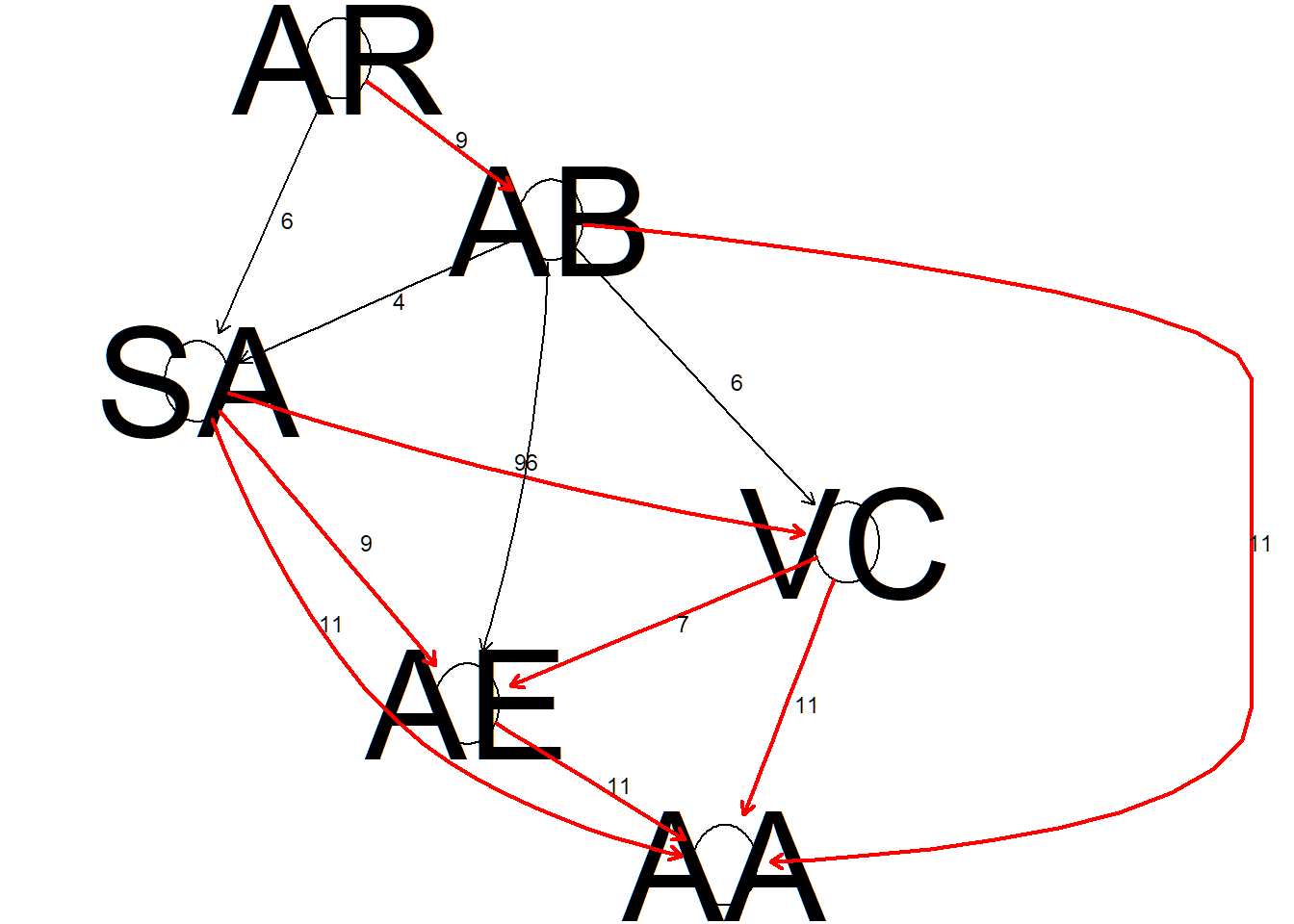
Let;s look at the results in the format of a table:
table <- net$arcs

kbl(table) %>%
  kable_classic(fixed_thead = T, full_width = T) %>%
  column_spec(1, bold = T, border_right = T) %>%
  column_spec(1:12, width = "30em", background = "white") %>%

  column_spec(13, color = "white",
background = spec_color(table$tot, end = 0.7, option="A"))| arcs | hc1 | hc2 | tabu1 | tabu2 | gs | iamb | fiamb | intamb | mmhc1 | mmhc2 | rsmax | tot |
|---|---|---|---|---|---|---|---|---|---|---|---|---|
| AB AA | 1 | 1 | 1 | 1 | 1.0 | 1.0 | 1.0 | 1.0 | 1 | 1 | 1 | 11 |
| AB AE | 1 | 1 | 1 | 1 | 0.5 | 0.5 | 0.5 | 0.5 | 0 | 0 | 0 | 6 |
| AB AR | 0 | 0 | 0 | 0 | 0.5 | 0.5 | 0.5 | 0.5 | 0 | 0 | 0 | 2 |
| AB SA | 1 | 1 | 1 | 1 | 0.0 | 0.0 | 0.0 | 0.0 | 0 | 0 | 0 | 4 |
| AB VC | 1 | 1 | 1 | 1 | 0.5 | 0.5 | 0.5 | 0.5 | 0 | 0 | 0 | 6 |
| AE AA | 1 | 1 | 1 | 1 | 1.0 | 1.0 | 1.0 | 1.0 | 1 | 1 | 1 | 11 |
| AE AB | 0 | 0 | 0 | 0 | 0.5 | 0.5 | 0.5 | 0.5 | 1 | 1 | 1 | 5 |
| AE SA | 0 | 0 | 0 | 0 | 0.5 | 0.5 | 0.5 | 0.5 | 0 | 0 | 0 | 2 |
| AE VC | 0 | 1 | 0 | 1 | 0.5 | 0.5 | 0.5 | 0.5 | 0 | 0 | 0 | 4 |
| AR AB | 1 | 1 | 1 | 1 | 0.5 | 0.5 | 0.5 | 0.5 | 1 | 1 | 1 | 9 |
| AR SA | 1 | 1 | 1 | 1 | 0.5 | 0.5 | 0.5 | 0.5 | 0 | 0 | 0 | 6 |
| AR VC | 0 | 1 | 0 | 1 | 0.5 | 0.5 | 0.5 | 0.5 | 0 | 0 | 0 | 4 |
| SA AA | 1 | 1 | 1 | 1 | 1.0 | 1.0 | 1.0 | 1.0 | 1 | 1 | 1 | 11 |
| SA AE | 1 | 1 | 1 | 1 | 0.5 | 0.5 | 0.5 | 0.5 | 1 | 1 | 1 | 9 |
| SA AR | 0 | 0 | 0 | 0 | 0.5 | 0.5 | 0.5 | 0.5 | 1 | 1 | 1 | 5 |
| SA VC | 1 | 1 | 1 | 1 | 0.5 | 0.5 | 0.5 | 0.5 | 1 | 1 | 1 | 9 |
| VC AA | 1 | 1 | 1 | 1 | 1.0 | 1.0 | 1.0 | 1.0 | 1 | 1 | 1 | 11 |
| VC AB | 0 | 0 | 0 | 0 | 0.5 | 0.5 | 0.5 | 0.5 | 1 | 1 | 1 | 5 |
| VC AE | 1 | 0 | 1 | 0 | 0.5 | 0.5 | 0.5 | 0.5 | 1 | 1 | 1 | 7 |
| VC AR | 0 | 0 | 0 | 0 | 0.5 | 0.5 | 0.5 | 0.5 | 1 | 1 | 1 | 5 |
| VC SA | 0 | 0 | 0 | 0 | 0.5 | 0.5 | 0.5 | 0.5 | 0 | 0 | 0 | 2 |
We are now able to derive the Bayesian network with the most robust arcs. The robust structure is defined by arcs that appear in a majority of learned networks. In other words, the links between the variables do not depend on the learning algorithm and is therefore considered robust.
x <- net$robust.net # x holds the robust network as derived from SBN_robustNet
arcs(x)             # 12
## from to
## [1,] "AE" "AA"
## [2,] "SA" "VC"
## [3,] "SA" "AE"
## [4,] "SA" "AA"
## [5,] "AR" "AB"
## [6,] "AB" "SA"
## [7,] "VC" "AE"
## [8,] "AB" "AA"
## [9,] "VC" "AA"
## [10,] "AB" "VC"
## [11,] "AB" "AE"
## [12,] "AR" "SA"score (x, datiBN) # Network score -19681.47## [1] -19681.47Let’s look at the corresponding centrality plot of the Bayesian network, with outdegree and indegree as centrality measures. Let’s also compare the centrality measures with those of the original model.
# Like the BN derived above, let's make a bn-object based on the original model
xdag <- empty.graph(nodes = c("AR", "AB", "SA","VC", "AE","AA"))
arc.set <- matrix(c("AR", "AB",
                    "AB", "SA",
                    "AB", "AE",
                    "SA", "AE",
                    "SA", "VC",
                    "AE", "VC",
                    "AE", "AA",
                    "VC", "AA"),
                    byrow = TRUE,
                    ncol = 2,
                    dimnames = list(NULL, c("from", "to")))
arcs(xdag) <- arc.set
Now we can compare the centralities of the original model by Rainville and Price with the centralities of our newly-learned model. This measure describes the standardized amount of incoming and outgoing edges, thereby providing a sense of which nodes in the model are the most central (i.e. a hub in the network).
# centralities original model
centr_original <- qgraph(xdag,DoNotPlot=T)
# centralities alternative model
centr_alternative <- qgraph(x,DoNotPlot=T)
centralityPlot(list(original = centr_original,
alternative = centr_alternative),
theme_bw = T, scale = "z-scores")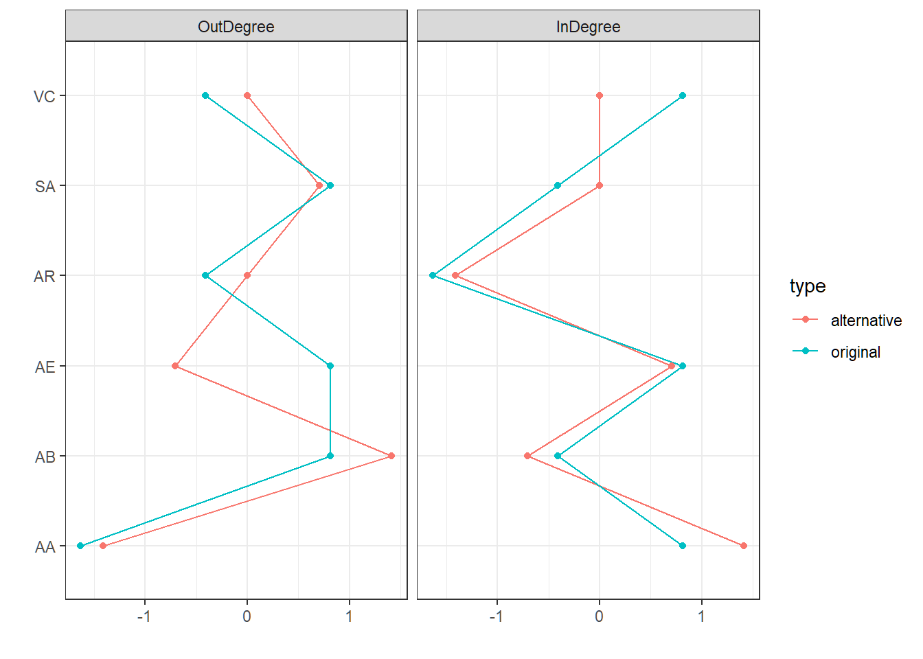 Additionally, we derive a Bayesian network with the proportion of occurrence of each arc in the bootstrap replicates.
set.seed(123)

R = 100
m = 100

ar  <- arcs(x) #arcs of the robust model
n.arcs <- dim(ar)[1] #29
ar  <- cbind(ar,paste(ar[,1],ar[,2]),paste(ar[,2],ar[,1]))
rep <- matrix(0,n.arcs,R)

for (i in 1:R){
  sam_bo <- datiBN[sample(c(1:dim(datiBN)[1]), m, replace = TRUE),]

  # check for appropriate algorithm selection based on the outcome of SBN_robustNet
    net.r <- hc(sam_bo,
                score     = "bic-g",
                blacklist = blacklist,
                debug     = FALSE)

  ar_s <- arcs(net.r)
  ar_s <- cbind(ar_s,paste(ar_s[,1],ar_s[,2]))
  rep[ar[,3]%in%ar_s[,3],i]<-1
  rep[ar[,4]%in%ar_s[,3],i]<-1
}

strength<-data.frame(ar[,1:2],apply(rep,1,mean))
strength
## from to apply.rep..1..mean.
## 1 AE AA 1.00
## 2 SA VC 1.00
## 3 SA AE 0.94
## 4 SA AA 0.79
## 5 AR AB 0.92
## 6 AB SA 0.30
## 7 VC AE 0.60
## 8 AB AA 0.45
## 9 VC AA 0.58
## 10 AB VC 0.42
## 11 AB AE 0.50
## 12 AR SA 0.10plot_s(x,strength)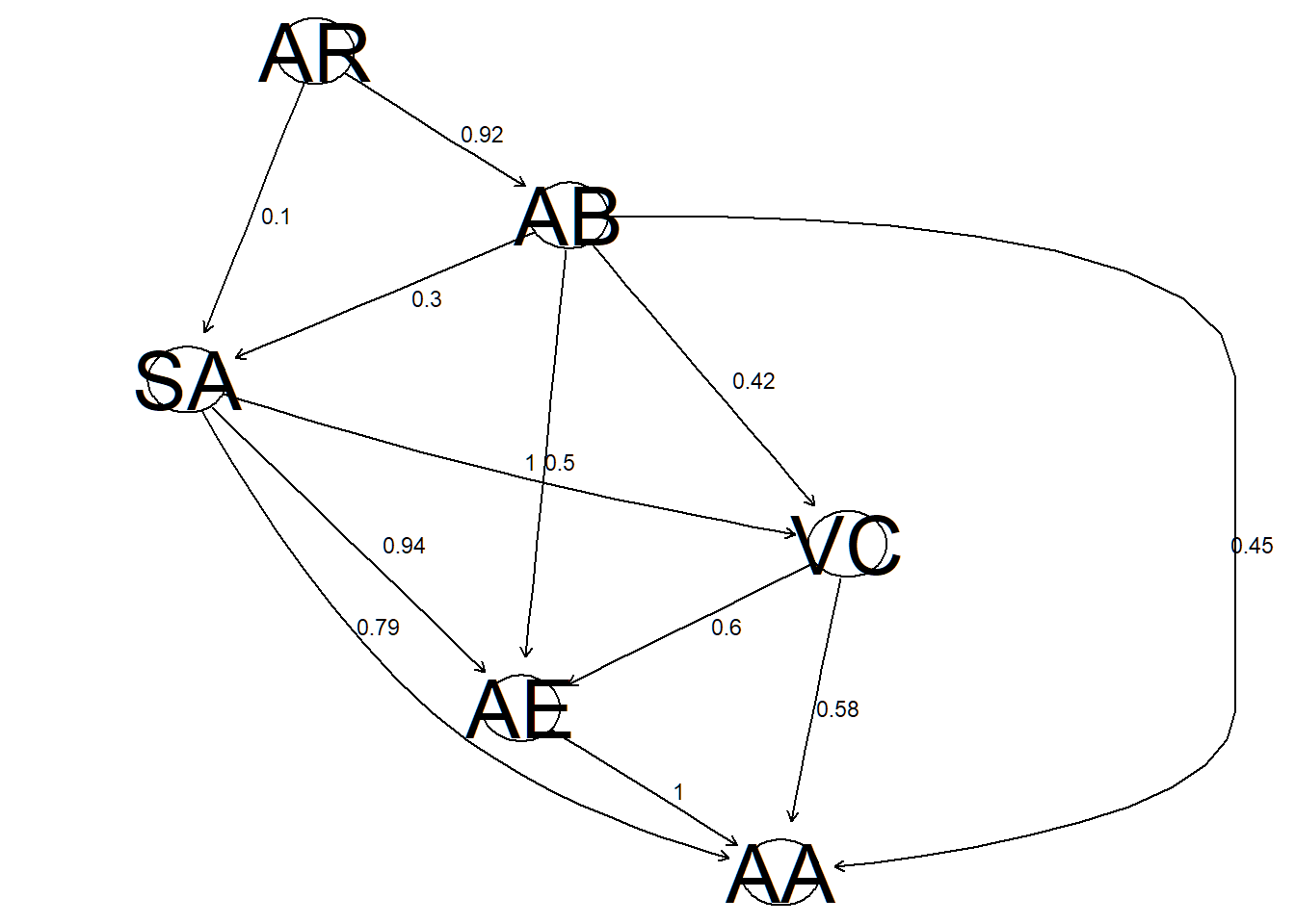
The following figure presents a heatmap of the Bauyesian network based on the index called distance-weighted influence (DWI) that orders the influence of all relevant nodes based on the network structure (see Albrecht et al., 2014). the further away a node is from the target node, the less is the influence of that node. The impact growswith the number of such paths (see also Cugnata et al., 2016).
Red indicates the target node (altered state of awareness) and the different shades of green of the remaining nodes indicate the proportion of their importance, i.e., less intense green suggests less influence. Here, absorption appears to have the largest impact (based on this index).
impo <- imp(x,target_node,strength)

plot_DWI(x, impo$importance, target_node)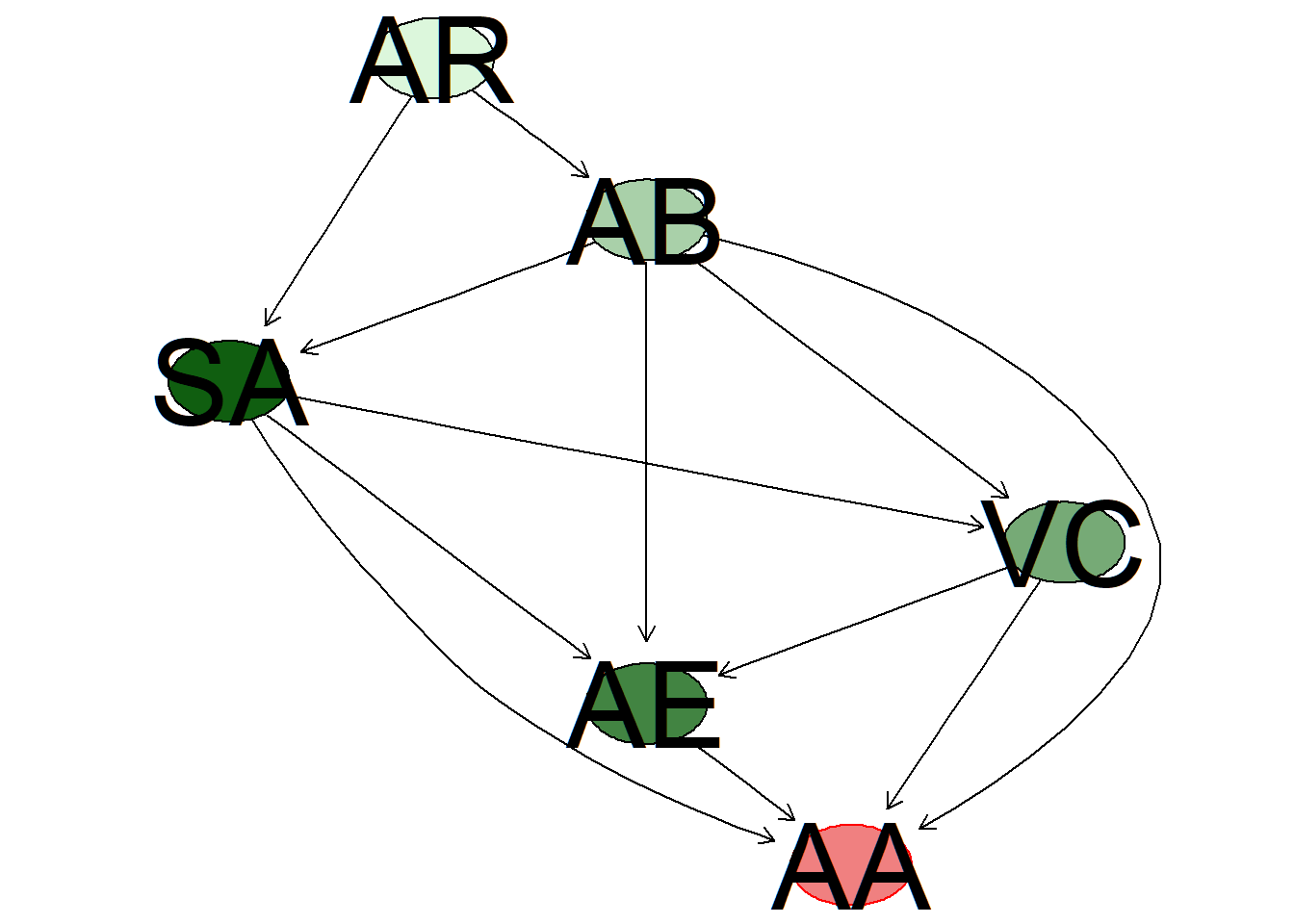
Convert the Bayesian network to a structural equation model (SEM):
paModel <- bnpa::gera.pa.model(x, datiBN)##
## Mounting a PA input model...pa.model.fit <- lavaan::sem(paModel, datiBN, std.lv = TRUE)The results of the SEM, including the standardized parameters:
lavaan::summary(pa.model.fit, rsquare = TRUE, standardized = TRUE, modindices = TRUE)## lavaan 0.6-12 ended normally after 1 iterations
##
## Estimator ML
## Optimization method NLMINB
## Number of model parameters 17
##
## Number of observations 2629
##
## Model Test User Model:
##
## Test statistic 7.972
## Degrees of freedom 3
## P-value (Chi-square) 0.047
##
## Parameter Estimates:
##
## Standard errors Standard
## Information Expected
## Information saturated (h1) model Structured
##
## Regressions:
## Estimate Std.Err z-value P(>|z|) Std.lv Std.all
## SA ~
## AR (c1) 0.107 0.020 5.332 0.000 0.107 0.107
## AB (c2) -0.262 0.020 -13.365 0.000 -0.262 -0.268
## AA ~
## SA (c3) -0.241 0.017 -14.125 0.000 -0.241 -0.235
## VC (c4) -0.187 0.017 -11.171 0.000 -0.187 -0.181
## AE (c5) 0.424 0.016 27.232 0.000 0.424 0.419
## AB (c6) 0.153 0.013 11.602 0.000 0.153 0.153
## VC ~
## SA (c7) 0.575 0.016 36.841 0.000 0.575 0.579
## AB (c8) -0.147 0.015 -9.614 0.000 -0.147 -0.151
## AE ~
## SA (c9) -0.368 0.020 -18.247 0.000 -0.368 -0.362
## VC (c10) -0.249 0.020 -12.201 0.000 -0.249 -0.244
## AB (c11) 0.149 0.016 9.161 0.000 0.149 0.150
## AB ~
## AR (c12) -0.399 0.018 -21.698 0.000 -0.399 -0.390
##
## Variances:
## Estimate Std.Err z-value P(>|z|) Std.lv Std.all
## .SA 0.897 0.025 36.256 0.000 0.897 0.895
## .AA 0.407 0.011 36.256 0.000 0.407 0.385
## .VC 0.581 0.016 36.256 0.000 0.581 0.588
## .AE 0.638 0.018 36.256 0.000 0.638 0.618
## .AB 0.886 0.024 36.256 0.000 0.886 0.848
##
## R-Square:
## Estimate
## SA 0.105
## AA 0.615
## VC 0.412
## AE 0.382
## AB 0.152
##
## Modification Indices:
##
## lhs op rhs mi epc sepc.lv sepc.all sepc.nox
## 1 SA ~~ AA 0.000 -0.002 -0.002 -0.003 -0.003
## 2 SA ~~ VC 4.199 -0.279 -0.279 -0.386 -0.386
## 3 SA ~~ AE 3.761 -0.277 -0.277 -0.366 -0.366
## 4 AA ~~ AB 0.000 0.000 0.000 0.001 0.001
## 5 VC ~~ AB 4.199 0.074 0.074 0.103 0.103
## 6 AE ~~ AB 3.761 0.073 0.073 0.098 0.098
## 7 SA ~ AA 0.076 -0.065 -0.065 -0.067 -0.067
## 8 SA ~ VC 4.199 -0.480 -0.480 -0.477 -0.477
## 9 SA ~ AE 1.994 -0.307 -0.307 -0.312 -0.312
## 10 AA ~ AR 0.000 0.000 0.000 0.000 0.000
## 11 VC ~ AR 4.199 0.033 0.033 0.033 0.034
## 12 AE ~ AR 3.761 0.033 0.033 0.032 0.033
## 13 AB ~ AA 0.076 0.017 0.017 0.017 0.017
## 14 AB ~ VC 4.199 0.127 0.127 0.124 0.124
## 15 AB ~ AE 1.994 0.081 0.081 0.081 0.081
## 16 AR ~ AA 0.076 0.008 0.008 0.008 0.008
## 17 AR ~ VC 4.199 0.057 0.057 0.057 0.057
## 18 AR ~ AE 1.994 0.037 0.037 0.037 0.037lavaan::standardizedSolution(pa.model.fit) ## lhs op rhs label est.std se z pvalue ci.lower ci.upper
## 1 SA ~ AR c1 0.107 0.020 5.370 0 0.068 0.146
## 2 SA ~ AB c2 -0.268 0.019 -13.788 0 -0.306 -0.230
## 3 AA ~ SA c3 -0.235 0.017 -14.216 0 -0.267 -0.203
## 4 AA ~ VC c4 -0.181 0.016 -11.205 0 -0.213 -0.150
## 5 AA ~ AE c5 0.419 0.015 28.279 0 0.390 0.448
## 6 AA ~ AB c6 0.153 0.013 11.590 0 0.127 0.178
## 7 VC ~ SA c7 0.579 0.013 43.805 0 0.553 0.605
## 8 VC ~ AB c8 -0.151 0.016 -9.663 0 -0.182 -0.120
## 9 AE ~ SA c9 -0.362 0.019 -18.919 0 -0.400 -0.325
## 10 AE ~ VC c10 -0.244 0.020 -12.380 0 -0.283 -0.205
## 11 AE ~ AB c11 0.150 0.016 9.214 0 0.118 0.182
## 12 AB ~ AR c12 -0.390 0.016 -24.510 0 -0.421 -0.359
## 13 SA ~~ SA 0.895 0.011 79.357 0 0.873 0.917
## 14 AA ~~ AA 0.385 0.012 32.727 0 0.362 0.408
## 15 VC ~~ VC 0.588 0.015 39.946 0 0.559 0.616
## 16 AE ~~ AE 0.618 0.015 41.510 0 0.589 0.647
## 17 AB ~~ AB 0.848 0.012 68.432 0 0.824 0.872
## 18 AR ~~ AR 1.000 0.000 NA NA 1.000 1.000We are of course also interested in model fit. We use the following selection of fit measures:
fitmeasures <- print(lavaan::fitMeasures(pa.model.fit, c("chisq", "df", "pvalue", "cfi","tli", "rmsea","rmsea.ci.lower","rmsea.ci.upper","rmsea.pvalue","srmr","gfi"), output = "text"), add.h0 = TRUE) %>% kbl() %>%
kable_classic(full_width = F) %>%
  column_spec(1, bold = T, border_right = T) %>%
  column_spec(1:2, background = "white")
##
## Model Test User Model:
##
## Test statistic 7.972
## Degrees of freedom 3
## P-value 0.047
##
## User Model versus Baseline Model:
##
## Comparative Fit Index (CFI) 0.999
## Tucker-Lewis Index (TLI) 0.996
##
## Root Mean Square Error of Approximation:
##
## RMSEA 0.025
## 90 Percent confidence interval - lower 0.003
## 90 Percent confidence interval - upper 0.047
## P-value RMSEA <= 0.05 0.971
##
## Standardized Root Mean Square Residual:
##
## SRMR 0.008
##
## Other Fit Indices:
##
## Goodness of Fit Index (GFI) 0.999
## To wrap the results together, we plot the experiential model of hypnosis as a SEM path model:
# define original layout of the experiential model
m <- matrix(c("AR" , NA   , NA  , NA,
              NA   , "AB", NA   , "SA",
              NA   , NA,  "VC"  , NA,
              NA   , "AE", NA   , "AA"), byrow = TRUE, 4, 4)

SEMmodel <- semPlot::semPaths(pa.model.fit,
                              whatLabels="std",
                              layout = m,
                              edge.label.cex=0.7,
                              borders = TRUE,
                              color  = "green",
edge.color = "black") 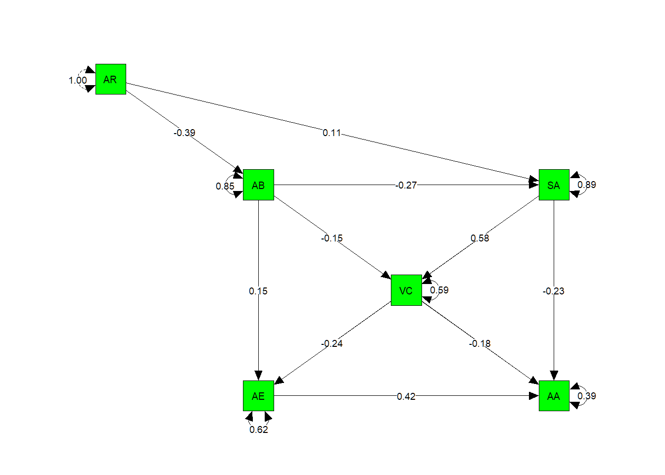
# Mark all parameter estimates by asterisks based on p-Values
p_pa2 <- semptools::mark_sig(SEMmodel, pa.model.fit)

#We can use mark_se() to add the standard errors for the parameter estimates
p_pa2 <- semptools::mark_se(p_pa2, pa.model.fit, sep = "\n")

my_curve_list <- c("AA ~ AB" = -2,
                   "AE ~ SA" = -2,
                   "AA ~ AE" = -2)

p_pa2 <- semptools::set_curve(p_pa2, my_curve_list)

plot(p_pa2)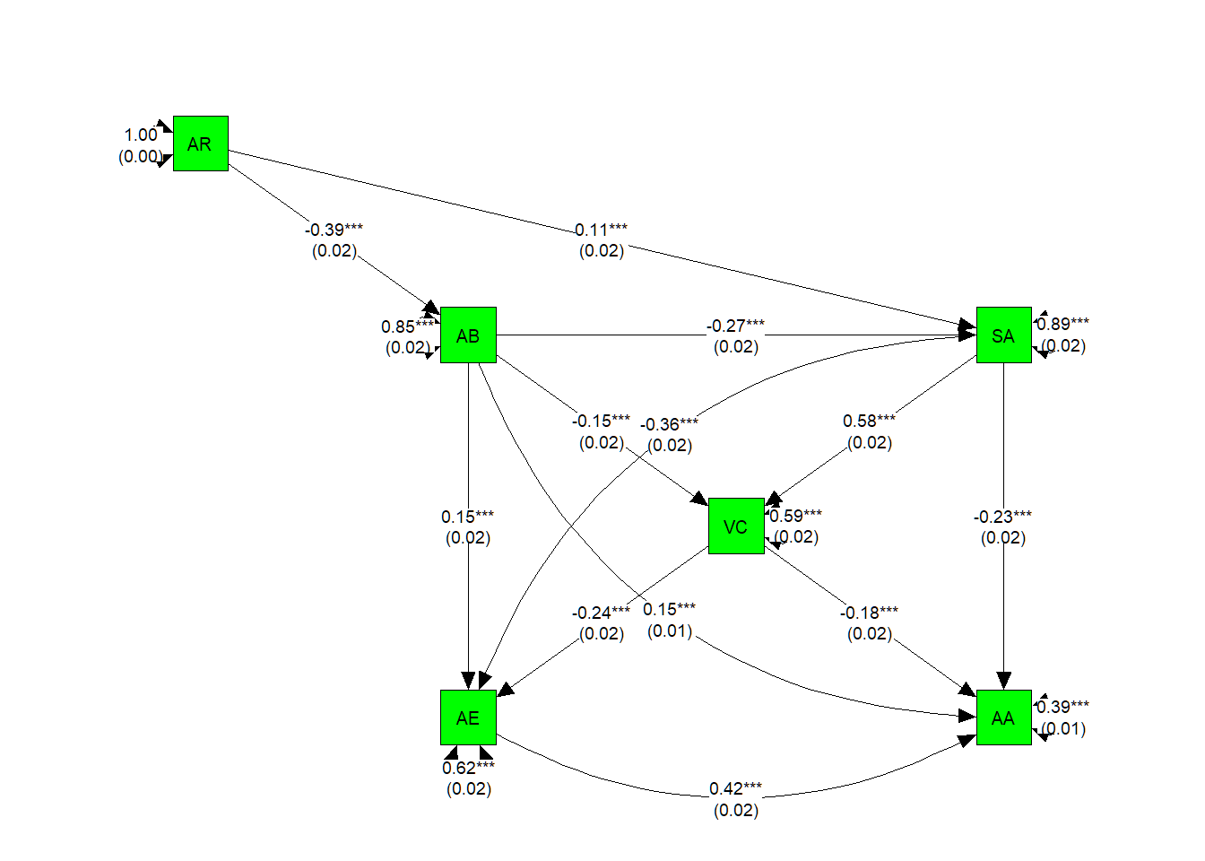
## see https://cran.r-project.org/web/packages/semptools/vignettes/semptools.htmlAnalysing spreading activation in path network
Finally, with the weighted path model in place, we can examine how the model functions when we activate specific variables and see how that effects the entire model in terms of spreading activation.
options(stringsAsFactors = FALSE)
set.seed(1234)

# Prepare network by making an appropriate igraph object
g_w_d <- igraph::as.igraph(SEMmodel, attributes = TRUE)

igraph::is_weighted(g_w_d) #TRUE
## [1] TRUEV(g_w_d)$name <- V(g_w_d)$label # ensure that the igraph object has a name attribute
#plot(g_w_d,
# edge.arrow.size = .2,
# edge.curved = .1)# Initial activation values
initial_df <-data.frame(node = c('AB', "AE"), activation = 50, stringsAsFactors = F)
initial_df## node activation
## 1 AB 50
## 2 AE 50# Simulation
result <- spreadr::spreadr(network = g_w_d,
start_run = initial_df, decay = 0.01,
retention = 0.9,
suppress = 0,
time = 20,
include_t0 = TRUE)
head(result, 10)## node activation time
## 1 SA 0.000 0
## 2 AA 0.000 0
## 3 VC 0.000 0
## 4 AE 50.000 0
## 5 AB 50.000 0
## 6 AR 0.000 0
## 7 SA 0.990 1
## 8 AA 3.465 1
## 9 VC 0.990 1
## 10 AE 45.540 1tail(result, 10)## node activation time
## 117 VC 2.945083 19
## 118 AE 9.434215 19
## 119 AB 5.580157 19
## 120 AR 0.000000 19
## 121 SA 2.209742 20
## 122 AA 10.874700 20
## 123 VC 2.792868 20
## 124 AE 8.671873 20
## 125 AB 4.971919 20
## 126 AR 0.000000 20# visualize the results
ggplot(data = result,
aes(x = time,
y = activation,
color = node,
group = node)) +
geom_point() + geom_line() + ggtitle('weighted, directed network') 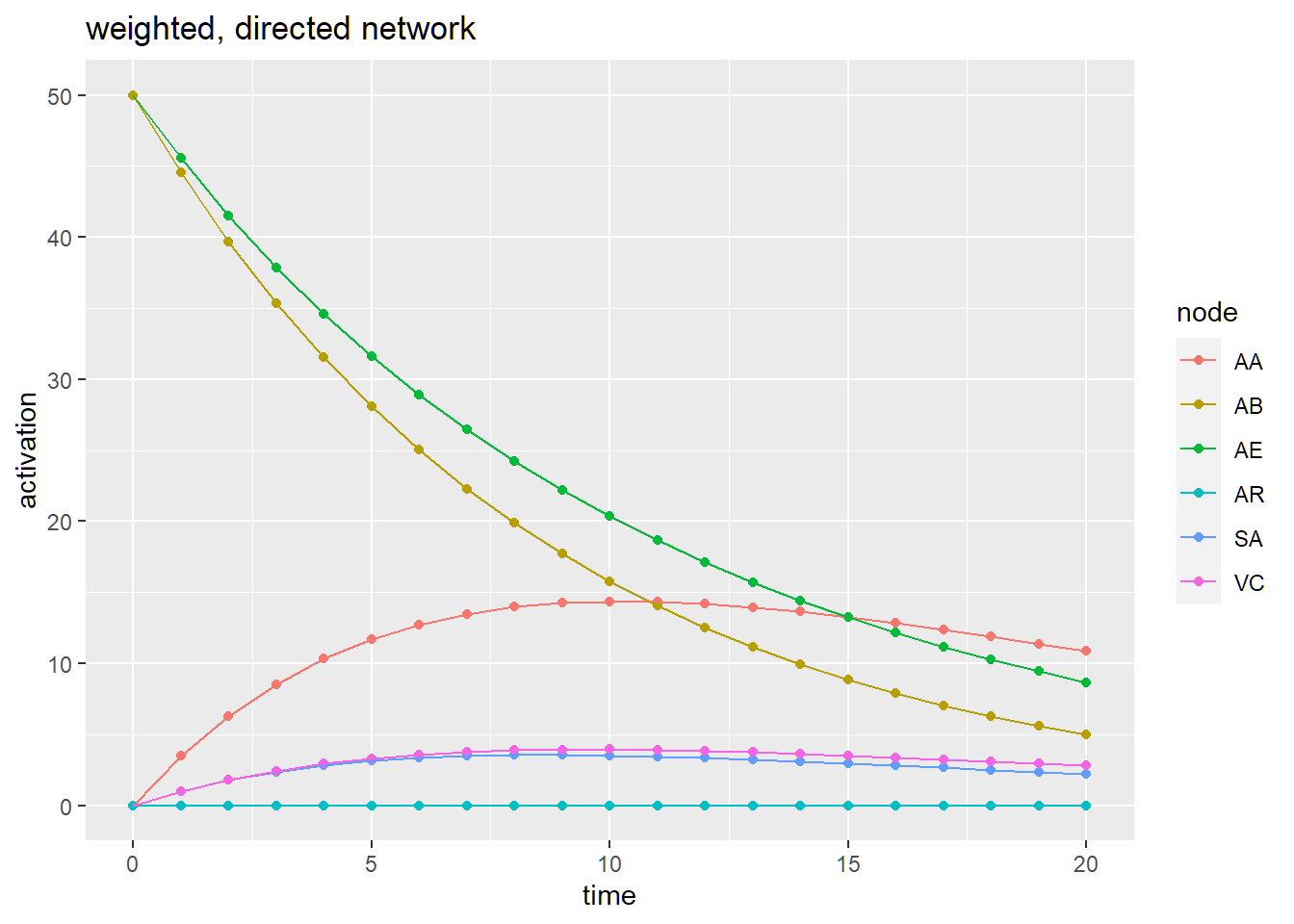
Conclusion
We obtained an excellent fit with our alternative model, compared to the fit measures of the original model. The analysis was based on a meta-analytic approach with several independent studies using various hypnotic induction-procedures.
That our new model fits better might not entirely come as a surprise, as it is precisely the purpose of the learning algorithms to find the best possible model that fits the data. However, it does provide us with insight into possible corrections to the original model which we might consider.
For instance, the original model appears to be too sparse (8 edges compared to 12 edges in the alternative model). Apparently, the interrelations between the dimensions of experience are more dense than hypothesized (i.e. the original model is a too simplistic model).
Also, when comparing the models, volitional control and altered experience (dissociation) swapped position. This change is represented in the comparison of node-centralities, where the outdegree of AE in the alternative model is much smaller than in the original model.
It might of interest to examine how our model fits to new data from a future study on the subjective experience of hypnosis.
Last, I want to thank all authors who provided me with the necessary summary data on the PCI!!
For data, source files and code only, see my github site as well Hypnosis
References
Albrecht, D., Nicholson, A. E., & Whittle, C. (2014). Structural Sensitivity for the Knowledge Engineering of Bayesian Networks. In Probabilistic Graphical Models, pp. 1–16. Basel, Switzerland: Springer International Publishing.
Cheung, M. W.-L. (2014). Fixed- and random-effects meta-analytic structural equation modeling: Examples and analyses in R. Behavior Research Methods, 46(1), 29–40. https://doi.org/10.3758/s13428-013-0361-y
Cheung, M. W.-L. (2015a). Meta-analysis: A structural equation modeling approach. John Wiley & Sons, Inc.
Cheung, M. W.-L. (2015b). metaSEM: An R package for meta-analysis using structural equation modeling. Frontiers in Psychology, 5(1521). https://doi.org/10.3389/fpsyg.2014.01521
Jak, S. (2015). Meta-analytic structural equation modelling. Springer, Utrecht, The Netherlands, 10.1007/978-3-319-27174-3
Kihlstrom, J.F. (2008). The domain of hypnosis, revisited. In: Nash, M.R., Barnier, A.J.(Eds.), The Oxford Handbook of Hypnosis: Theory, Research and Practice. Oxford University Press, Oxford; New York.
Nash, M. R. (2008). Foundations of clinical hypnosis. In M. R. Nash & A. J. Barnier (Eds.), The Oxford handbook of hypnosis: Theory, research, and practice (pp. 487-502). Oxford: Oxford University Press.
Rainville, P., & Price, D. D. (2003). Hypnosis phenomenology and the neurobiology ofconsciousness. International Journal of Clinical and Experimental Hypnosis, 51(2), 105–129
Thompson, J. M., Waelde, L. C., Tisza, K., & Spiegel, D. (2016). Hypnosis and mindfulness: Experiential and neurophysiological relationships. In Raz, A. & Lifshitz, M. (Eds.), Hypnosis and meditation: Towards an integrative science of conscious planes (pp. 129–142). Oxford University Press, Oxford, UK.
The studies from which the data came from:
Költő, A. (2015). Hypnotic Susceptibility and Mentalization Skills in the Context of Parental Behavior. Dissertation, Eötvös Loránd University, Hungary
Kumar, V. K., & Pekala, R. J. (1988). Hypnotizability, absorption, and individual differences in phenomenological experience. International Journal of Clinical and Experimental Hypnosis, 36, 80-88.
Kumar, V., Pekala, R. J., & Cummings, J. (1996). Trait factors, state effects, and hypnotizability. International Journal of Clinical and Experimental Hypnosis, 44(3), 232-249.
Loi,N.M. (2011). Absorption, Fantasy Proneness, and Trance: Dissociative Pathways of Affective Self-Regulation in Trauma. Dissertation, University of New England, Australia.
Pekala, R. J., Forbes, E., &: Contrisciani, P. A. (1989). Assessing the phenomenological effects of several stress management strategies. Imagination, Cognition, and Personality, 88, 265-28l.
Varga, K., Józsa, E., & Kekecs, Z. (2014). Comparative analysis of phenomenological patterns of hypnotists and subjects: An interactional perspective. Psychology of Consciousness:Theory, Research, and Practice, 1(3), 308-319.
Terhune, D. B., & Cardeña, E. (2010). Differential patterns of spontaneous experiential response to a hypnotic induction: A latent profile analysis. Consciousness and cognition, 19(4), 1140-1150.